Step-by-step PhAST problem setup¶

This notebook builds a small single-edge-notched tension problem from first principles. It creates and inspects the geometry and mesh, defines the material and boundary-value problem with the fluent Python API, writes a runnable schema-v1 YAML configuration, performs a bounded two-step CPU solve, and inspects the resulting artifacts.

Learning objectives:

Create a Gmsh .geo file and convert it to a .msh mesh.
Verify physical groups before using them as PhAST regions.
Apply material parameters, initial-condition choices, supports, and prescribed loading.
Distinguish the fluent authoring representation from the runnable YAML contract.
Run a short quasi-static phase-field workflow check and inspect the generated output directory.
Locate final field images, histories, trajectory stores, and optional animations.

Guided activity pattern:

Predict: identify the constrained and loaded boundaries and anticipate the displacement direction before running a cell.
Run and inspect: compare the generated mesh, physical groups, solver route, and result manifest with that prediction.
Change one quantity: modify h_bulk, l0, or u_top individually; do not change all three at once.
Explain: state which discretization, constitutive, or loading choice changed and which output should respond.
Fallback: if installation or execution is unavailable, use the rendered cell outputs and continue with the retained-results notebook.

The default run is intentionally short and is not crack-growth validation. For a research calculation, start from the closest checked-in example, refine the mesh, select a documented loading schedule, and retain the full result and provenance bundle.

Problem statement before software¶

The specimen is a two-dimensional notched plate subjected to a prescribed vertical displacement. The unknown fields are the displacement u and the phase-field damage variable d, where d = 0 denotes intact material and d = 1 denotes fully developed damage under the adopted convention.

For a quasi-static staggered increment, the computational sequence is:

Hold the current damage field fixed and solve mechanical equilibrium for displacement.
Update the tensile history quantity used to enforce irreversible crack driving.
Hold that driving state fixed and solve the regularized damage subproblem.
Repeat the displacement and damage updates until the selected staggered stopping criterion is met.
Write the accepted state and provenance artifacts.

In variational form, the displacement update seeks stationarity of the mechanical contribution with the damage field fixed, while the damage update seeks stationarity of the fracture contribution and degraded tensile energy with the mechanical driving state fixed. Finite-element test functions convert these statements into discrete residual equations. See the phase-field primer for the governing energies and the solver overview for the implemented pathways.

This notebook uses only two load steps so that a new user can inspect the complete software pathway. It establishes configuration and execution behaviour; it does not establish crack initiation, propagation, mesh convergence, or agreement with an experiment.

Predict before continuing: Which named boundary should remove rigid vertical motion? Which boundary should carry the prescribed displacement? Where should the initial notch appear in the setup plot?

1. Install dependencies¶

Run this cell in Colab. In a local clone, install PhAST with pip install -e . from the repository root and skip the Colab-specific package installation if your environment is already configured.

The Colab route checks out the published v0.16.2-arxiv.2606.23458 release rather than the mutable default branch. It rejects a cached checkout whose origin, commit, or tracked files do not match the expected release and prints the resolved commit for the session record.

The notebook uses Gmsh to create mesh.msh, MeshIO to inspect physical groups, Matplotlib and Pillow for visual checks, and PhAST for solving and result inspection.

import os
import sys
import subprocess
from pathlib import Path

IN_COLAB = "google.colab" in sys.modules
PHAST_REPOSITORY = "https://github.com/CEMS-Lab/PhAST.git"
PHAST_REVISION = "v0.16.2-arxiv.2606.23458"

if IN_COLAB:
    subprocess.run(["apt-get", "update", "-qq"], check=True)
    subprocess.run(["apt-get", "install", "-y", "-qq", "gmsh", "ffmpeg"], check=True)

    checkout = Path("/content") / f"PhAST-{PHAST_REVISION}"
    if checkout.exists():
        if not (checkout / ".git").is_dir():
            raise RuntimeError(
                f"{checkout} exists but is not a Git checkout. "
                "Restart the runtime or remove that directory explicitly."
            )
        origin = subprocess.check_output(
            ["git", "-C", str(checkout), "config", "--get", "remote.origin.url"],
            text=True,
        ).strip()
        if origin != PHAST_REPOSITORY:
            raise RuntimeError(
                f"Cached checkout origin is {origin!r}, expected {PHAST_REPOSITORY!r}."
            )
    else:
        subprocess.run(
            [
                "git",
                "clone",
                "--branch",
                PHAST_REVISION,
                "--depth",
                "1",
                PHAST_REPOSITORY,
                str(checkout),
            ],
            check=True,
        )

    subprocess.run(
        [
            "git",
            "-C",
            str(checkout),
            "fetch",
            "--depth",
            "1",
            "origin",
            f"refs/tags/{PHAST_REVISION}:refs/tags/{PHAST_REVISION}",
        ],
        check=True,
    )
    expected_commit = subprocess.check_output(
        ["git", "-C", str(checkout), "rev-list", "-n", "1", PHAST_REVISION],
        text=True,
    ).strip()
    resolved_commit = subprocess.check_output(
        ["git", "-C", str(checkout), "rev-parse", "HEAD"],
        text=True,
    ).strip()
    tracked_changes = subprocess.check_output(
        [
            "git",
            "-C",
            str(checkout),
            "status",
            "--porcelain",
            "--untracked-files=no",
        ],
        text=True,
    ).strip()
    if resolved_commit != expected_commit or tracked_changes:
        raise RuntimeError(
            "Cached PhAST checkout does not match the documented release. "
            "Restart the Colab runtime before continuing."
        )

    print(f"PhAST release: {PHAST_REVISION}")
    print(f"Resolved commit: {resolved_commit}")
    subprocess.run(
        [
            sys.executable,
            "-m",
            "pip",
            "install",
            "-q",
            "-e",
            str(checkout),
            "meshio",
            "matplotlib",
            "zarr",
            "h5py",
            "pyyaml",
        ],
        check=True,
    )
    os.chdir(checkout)
else:
    print(
        "Local run: use an activated PhAST environment and start Jupyter "
        "from the repository checkout."
    )

Local run: use an activated PhAST environment and start Jupyter from the repository checkout.

2. Imports and working directory¶

All generated files go into runs/notebook_sent/. Keeping the generated geometry, mesh, configuration, and results in one directory makes the run easy to archive or remove.

import json
import shutil
import textwrap

from PIL import Image as PILImage
import matplotlib.pyplot as plt
import meshio
import numpy as np
import yaml

here = Path.cwd().resolve()
repo_root = next(
    (candidate for candidate in (here, *here.parents)
     if (candidate / "pyproject.toml").is_file() and (candidate / "src" / "phast").is_dir()),
    here,
)
source_src = repo_root / "src"
if source_src.is_dir():
    sys.path.insert(0, str(source_src))
    os.environ["PYTHONPATH"] = str(source_src) + os.pathsep + os.environ.get("PYTHONPATH", "")

import phast

run_dir = (repo_root / "runs" / "notebook_sent").resolve()
run_dir.mkdir(parents=True, exist_ok=True)

geo_path = run_dir / "mesh.geo"
mesh_path = run_dir / "mesh.msh"
spec_path = run_dir / "authored_problem_spec.yaml"
config_path = run_dir / "config.yaml"
output_dir = run_dir / "results"

print("PhAST:", getattr(phast, "__version__", "source checkout"))
print("Repository root:", repo_root)
print("Working directory:", run_dir)

PhAST: source checkout
Repository root: /home/runner/work/PhAST/PhAST
Working directory: /home/runner/work/PhAST/PhAST/runs/notebook_sent

3. Define a small geometry¶

The geometry is a rectangular plate with a thin single-edge notch cut from the left boundary to mid-plate. The notch boundary is a named physical curve that supplies nodes for the initial damage field. This makes the geometry robust in Gmsh while still representing a pre-existing crack seed for the phase-field solve.

The physical names are the contract between the mesh and PhAST:

Name	Meaning	Used for
`body`	2D plate surface	material assignment
`bottom`	bottom edge	fixed support
`top`	top edge	prescribed vertical displacement
`notch`	embedded crack line	initial damage seed
`left`, `right`	side edges	optional inspection/output regions

L = 1.0          # plate width [mm]
H = 1.0          # plate height [mm]
a0 = 0.50        # initial notch/crack length [mm]
y_crack = 0.50   # crack vertical location [mm]
notch_gap = 0.012 # small geometric opening used for robust meshing [mm]
h_bulk = 0.08    # coarse element size [mm]
h_crack = 0.02   # local element size near the crack [mm]

geo_text = f"""
SetFactory("OpenCASCADE");

L = {L};
H = {H};
a0 = {a0};
yc = {y_crack};
g = {notch_gap};
h_bulk = {h_bulk};
h_crack = {h_crack};

Point(1) = {{0, 0, 0, h_bulk}};
Point(2) = {{L, 0, 0, h_bulk}};
Point(3) = {{L, H, 0, h_bulk}};
Point(4) = {{0, H, 0, h_bulk}};
Point(5) = {{0, yc + 0.5*g, 0, h_crack}};
Point(6) = {{a0, yc + 0.5*g, 0, h_crack}};
Point(7) = {{a0, yc - 0.5*g, 0, h_crack}};
Point(8) = {{0, yc - 0.5*g, 0, h_crack}};

Line(1) = {{1, 2}};
Line(2) = {{2, 3}};
Line(3) = {{3, 4}};
Line(4) = {{4, 5}};
Line(5) = {{5, 6}};
Line(6) = {{6, 7}};
Line(7) = {{7, 8}};
Line(8) = {{8, 1}};

Curve Loop(10) = {{1, 2, 3, 4, 5, 6, 7, 8}};
Plane Surface(20) = {{10}};

Field[1] = Distance;
Field[1].CurvesList = {{5, 6, 7}};
Field[2] = Threshold;
Field[2].InField = 1;
Field[2].SizeMin = h_crack;
Field[2].SizeMax = h_bulk;
Field[2].DistMin = 0.02;
Field[2].DistMax = 0.18;
Background Field = 2;

Physical Surface("body") = {{20}};
Physical Curve("bottom") = {{1}};
Physical Curve("right") = {{2}};
Physical Curve("top") = {{3}};
Physical Curve("left") = {{4, 8}};
Physical Curve("notch") = {{5, 6, 7}};
""".strip()

geo_path.write_text(geo_text + "\n", encoding="utf-8")
print(geo_path)
print(geo_text[:600] + "\n...")

/home/runner/work/PhAST/PhAST/runs/notebook_sent/mesh.geo
SetFactory("OpenCASCADE");

L = 1.0;
H = 1.0;
a0 = 0.5;
yc = 0.5;
g = 0.012;
h_bulk = 0.08;
h_crack = 0.02;

Point(1) = {0, 0, 0, h_bulk};
Point(2) = {L, 0, 0, h_bulk};
Point(3) = {L, H, 0, h_bulk};
Point(4) = {0, H, 0, h_bulk};
Point(5) = {0, yc + 0.5*g, 0, h_crack};
Point(6) = {a0, yc + 0.5*g, 0, h_crack};
Point(7) = {a0, yc - 0.5*g, 0, h_crack};
Point(8) = {0, yc - 0.5*g, 0, h_crack};

Line(1) = {1, 2};
Line(2) = {2, 3};
Line(3) = {3, 4};
Line(4) = {4, 5};
Line(5) = {5, 6};
Line(6) = {6, 7};
Line(7) = {7, 8};
Line(8) = {8, 1};

Curve Loop(10) = {1, 2, 3, 4, 5, 6, 7, 8};
Plane Surface(20) = 
...

4. Visualize the geometry before meshing¶

This schematic is not the finite-element mesh. It is a cheap sanity check: dimensions, crack location, and loaded/support boundaries should be correct before generating elements.

fig, ax = plt.subplots(figsize=(6, 5))
ax.plot([0, L, L, 0, 0], [0, 0, H, H, 0], color="0.15", lw=2)
ax.fill([0, a0, a0, 0], [y_crack - notch_gap/2, y_crack - notch_gap/2, y_crack + notch_gap/2, y_crack + notch_gap/2], color="crimson", alpha=0.22)
ax.plot([0, a0], [y_crack, y_crack], color="crimson", lw=3, label="initial notch / damage seed")
ax.plot([0, L], [0, 0], color="royalblue", lw=4, label="fixed bottom")
ax.plot([0, L], [H, H], color="darkorange", lw=4, label="prescribed top displacement")
ax.set_aspect("equal")
ax.set_xlabel("x [mm]")
ax.set_ylabel("y [mm]")
ax.set_title("Geometry and named boundaries")
ax.legend(loc="upper center", bbox_to_anchor=(0.5, -0.12), ncol=1)
fig.tight_layout()
fig.savefig(run_dir / "geometry_preview.png", dpi=180)
plt.show()

5. Generate the mesh with Gmsh¶

The command below converts mesh.geo into mesh.msh. If this fails in a local environment, install Gmsh and make sure the gmsh executable is on PATH.

gmsh = shutil.which("gmsh")
if gmsh is None:
    raise RuntimeError("gmsh executable was not found on PATH")

cmd = [gmsh, "-2", str(geo_path), "-format", "msh2", "-o", str(mesh_path)]
print(" ".join(cmd))
subprocess.run(cmd, check=True)
print(mesh_path, mesh_path.stat().st_size, "bytes")

/opt/hostedtoolcache/Python/3.11.16/x64/bin/gmsh -2 /home/runner/work/PhAST/PhAST/runs/notebook_sent/mesh.geo -format msh2 -o /home/runner/work/PhAST/PhAST/runs/notebook_sent/mesh.msh

Info    : Running '/opt/hostedtoolcache/Python/3.11.16/x64/bin/gmsh -2 /home/runner/work/PhAST/PhAST/runs/notebook_sent/mesh.geo -format msh2 -o /home/runner/work/PhAST/PhAST/runs/notebook_sent/mesh.msh' [Gmsh 4.15.2, 1 node, max. 1 thread]
Info    : Started on Mon Sep 21 22:43:50 2026
Info    : Reading '/home/runner/work/PhAST/PhAST/runs/notebook_sent/mesh.geo'...
Info    : Done reading '/home/runner/work/PhAST/PhAST/runs/notebook_sent/mesh.geo'
Info    : Meshing 1D...
Info    : [  0%] Meshing curve 1 (Line)
Info    : [ 20%] Meshing curve 2 (Line)
Info    : [ 30%] Meshing curve 3 (Line)
Info    : [ 40%] Meshing curve 4 (Line)
Info    : [ 60%] Meshing curve 5 (Line)
Info    : [ 70%] Meshing curve 6 (Line)
Info    : [ 80%] Meshing curve 7 (Line)
Info    : [ 90%] Meshing curve 8 (Line)
Info    : Done meshing 1D (Wall 0.00342108s, CPU 0.002153s)
Info    : Meshing 2D...
Info    : Meshing surface 20 (Plane, Frontal-Delaunay)
Info    : Done meshing 2D (Wall 0.021159s, CPU 0.021159s)
Info    : 688 nodes 1382 elements
Info    : Writing '/home/runner/work/PhAST/PhAST/runs/notebook_sent/mesh.msh'...
Info    : Done writing '/home/runner/work/PhAST/PhAST/runs/notebook_sent/mesh.msh'
Info    : Stopped on Mon Sep 21 22:43:50 2026 (From start: Wall 0.0292189s, CPU 0.260933s)
/home/runner/work/PhAST/PhAST/runs/notebook_sent/mesh.msh 61254 bytes

6. Inspect named regions from the mesh¶

This is the most important mesh validation step. The solver can only apply materials, initial conditions, supports, loads, and histories to regions that are present in the mesh. Missing or misspelled physical names should be fixed in the .geo file before running.

mesh_summary = phast.inspect_mesh(mesh_path)
print("points:", mesh_summary["n_points"])
print("cell blocks:", mesh_summary["cells"])
print(json.dumps(mesh_summary["named_groups"], indent=2))

required_groups = {"body", "bottom", "top", "notch"}
missing = required_groups - set(mesh_summary["named_groups"])
if missing:
    raise RuntimeError(f"Missing required physical groups: {sorted(missing)}")

points: 688
cell blocks: [{'type': 'line', 'count': 114, 'nodes_per_cell': 2}, {'type': 'triangle', 'count': 1260, 'nodes_per_cell': 3}]
{
  "body": {
    "id": 1,
    "dimension": 2,
    "cell_counts": {
      "triangle": 1260
    }
  },
  "bottom": {
    "id": 2,
    "dimension": 1,
    "cell_counts": {
      "line": 13
    }
  },
  "left": {
    "id": 5,
    "dimension": 1,
    "cell_counts": {
      "line": 24
    }
  },
  "notch": {
    "id": 6,
    "dimension": 1,
    "cell_counts": {
      "line": 51
    }
  },
  "right": {
    "id": 3,
    "dimension": 1,
    "cell_counts": {
      "line": 13
    }
  },
  "top": {
    "id": 4,
    "dimension": 1,
    "cell_counts": {
      "line": 13
    }
  }
}

7. Visualize the mesh and physical groups¶

A visual check catches common mistakes: swapped top/bottom groups, an unembedded crack line, very coarse crack-tip resolution, or an accidental empty surface group.

mesh = meshio.read(mesh_path)
points = mesh.points[:, :2]

triangles = []
lines = []
line_tags = []
for block_index, block in enumerate(mesh.cells):
    if block.type == "triangle":
        triangles.append(block.data)
    if block.type == "line":
        lines.append(block.data)
        tags = mesh.cell_data.get("gmsh:physical", [])[block_index]
        line_tags.append(tags)

triangles = np.vstack(triangles) if triangles else np.empty((0, 3), dtype=int)
lines = np.vstack(lines) if lines else np.empty((0, 2), dtype=int)
line_tags = np.concatenate(line_tags) if line_tags else np.empty((0,), dtype=int)

id_to_name = {int(data[0]): name for name, data in mesh.field_data.items()}
colors = {"bottom": "royalblue", "top": "darkorange", "left": "0.35", "right": "0.35", "notch": "crimson"}

fig, ax = plt.subplots(figsize=(7, 6))
if len(triangles):
    ax.triplot(points[:, 0], points[:, 1], triangles, color="0.82", linewidth=0.5)
for edge, tag in zip(lines, line_tags):
    name = id_to_name.get(int(tag), str(tag))
    xy = points[edge]
    ax.plot(xy[:, 0], xy[:, 1], color=colors.get(name, "0.4"), lw=2.0 if name == "notch" else 1.4)
ax.set_aspect("equal")
ax.set_xlabel("x [mm]")
ax.set_ylabel("y [mm]")
ax.set_title("Mesh with named physical curves")
fig.tight_layout()
fig.savefig(run_dir / "mesh_preview.png", dpi=180)
plt.show()

8. Build the problem manually with `phast.Problem`¶

The fluent API is best while designing a model because each line corresponds to a physical decision. The region names on the left are the names used by this Python model; the from_mesh values are the physical names stored in mesh.msh.

The short run below uses AT2 damage, the spectral split, a quasi-static staggered solve, and CPU execution. The geometric notch is present in the mesh. Full damage pre-seeding is shown as an opt-in switch because it is useful for full fracture studies but can be too severe for a two-step Colab smoke test. Change only one choice at a time when exploring a new model.

num_steps = 2          # quick tutorial run; increase for smoother damage evolution
u_top = 0.0002         # prescribed final displacement [mm]
l0 = 0.04             # phase-field length scale [mm]
enable_damage_preseed = False

problem = (
    phast.Problem("Notebook SENT tutorial")
    .mesh(str(mesh_path))
    .region("body", kind="domain", from_mesh="body")
    .region("bottom", from_mesh="bottom")
    .region("top", from_mesh="top")
    .region("notch", from_mesh="notch")
    .material(
        "glass",
        region="body",
        E=210000.0,
        nu=0.3,
        Gc=2.7,
        l0=l0,
        rho=7.8e-09,
        eta_residual=1.0e-07,
        energy_split="spectral",
        pf_model="AT2",
        plane_stress=False,
    )
    .boundary_condition("fix", region="bottom", dof="x", name="fix_bottom_x")
    .boundary_condition("fix", region="bottom", dof="y", name="fix_bottom_y")
    .boundary_condition("displacement", region="top", dof="y", value=1.0, name="pull_top")
    .analysis_step(
        "load",
        kind="quasi_static",
        controls={"protocol": "simple", "num_steps": num_steps, "dt": u_top / num_steps},
        active_boundary_conditions=["fix_bottom_x", "fix_bottom_y", "pull_top"],
    )
    .solver(
        "quasi_static",
        stagger_tol=1.0e-6,
        max_stagger=50,
        preconditioner="jacobi",
        damage_tol=1.0e-5,
        static_tol=1.0e-7,
        damage_max_iter=500,
        static_max_iter=500,
        fail_on_mechanics_nonconvergence=False,
        fail_on_stagger_nonconvergence=False,
        backend="auto",
        device="cpu",
    )
    .outputs(
        fields=[{"name": "trajectory", "every": 1, "format": "zarr"}],
        histories=[{"name": "reaction_force", "region": "bottom", "dof": "y"}],
        plots=True,
        profile=True,
        gif=True,
        gif_frames=24,
        gif_fields="damage",
        animation_format="gif",
        print_every=1,
    )
)

if enable_damage_preseed:
    problem.initial_condition("damage", region="notch", value=1.0)

problem.validate_setup()

{'mesh': '/home/runner/work/PhAST/PhAST/runs/notebook_sent/mesh.msh',
 'regions': {'body': {'source': 'named_group',
   'external_name': 'body',
   'dimension': 2,
   'cell_counts': {'triangle': 1260}},
  'bottom': {'source': 'named_group',
   'external_name': 'bottom',
   'dimension': 1,
   'cell_counts': {'line': 13}},
  'top': {'source': 'named_group',
   'external_name': 'top',
   'dimension': 1,
   'cell_counts': {'line': 13}},
  'notch': {'source': 'named_group',
   'external_name': 'notch',
   'dimension': 1,
   'cell_counts': {'line': 51}}}}

9. Visualize supports, loading, and the damage seed¶

problem.plot_setup(...) writes a static setup preview. The extra overlay below explicitly marks the prescribed displacement and the seeded crack so the notebook remains readable even if the default preview style changes.

setup_preview = run_dir / "initial_conditions.png"
problem.plot_setup(output=setup_preview)

img = np.asarray(PILImage.open(setup_preview).convert("RGB"))
fig, ax = plt.subplots(figsize=(8, 5))
ax.imshow(img)
ax.axis("off")
ax.set_title("PhAST setup preview")
plt.show()
print(setup_preview)

/home/runner/work/PhAST/PhAST/runs/notebook_sent/initial_conditions.png

10. Solver settings: what the common choices mean¶

Phase-field fracture replaces a sharp crack with a continuous damage field d. Values near 0 represent intact material and values near 1 represent fully damaged material. The length scale l0 controls the width of the diffuse crack band, so the mesh should resolve l0 near the expected crack path.

Choice	Typical values	Meaning
`pf_model`	`AT1`, `AT2`	Crack-density model. AT2 is smooth at damage onset; AT1 has a finite damage threshold and is common in dynamic benchmark decks.
`energy_split`	`spectral`, `amor`, `isotropic`, `star_convex`	How tensile and compressive elastic energy contributions are separated before driving damage. Use the split required by the benchmark or paper claim.
`solver_type`	`quasi_static`, `explicit`	Quasi-static solves coupled displacement/damage equilibrium at each load increment. Explicit dynamics advances the transient wave/crack problem with a stable time step.
static vs dynamic	`quasi_static` vs `explicit`	Static/quasi-static cases ignore inertia; dynamic cases require density and time-step controls.
implicit vs explicit	`quasi_static` uses iterative equilibrium solves; `explicit` uses time stepping	Current public examples promote quasi-static fracture and explicit dynamic fracture. Experimental or beta paths should stay clearly labelled.
trajectory format	`zarr`, `h5`, `both`	Zarr is preferred for public runs; HDF5 is retained for compatibility with older post-processing scripts.

For a paper result, keep these choices in YAML and report them in the run manifest. Do not rely on notebook state as the only record of a simulation.

11. Write the runnable YAML configuration¶

The fluent Problem object is useful for authoring and setup validation. Its saved schema-v2 specification is an inspection representation and does not imply that every combination has a promoted execution adapter. This cell retains that specification separately, then writes the supported schema-v1 YAML fields used by the public fracture runner.

problem.save(spec_path)

execution_config = {
    "schema_version": 1,
    "problem": {
        "name": "Notebook SENT workflow check",
        "reference": "Educational setup; not a validation benchmark",
    },
    "geometry": {"mesh_path": str(mesh_path)},
    "material": {
        "E": 210000.0,
        "nu": 0.3,
        "Gc": 2.7,
        "l0": l0,
        "rho": 7.8e-09,
        "eta_residual": 1.0e-07,
        "energy_split": "spectral",
        "pf_model": "AT2",
        "plane_stress": False,
    },
    "boundary_conditions": [
        {"nodes": "bottom", "type": "fix", "component": 0, "value": 0.0},
        {"nodes": "bottom", "type": "fix", "component": 1, "value": 0.0},
        {"nodes": "top", "type": "prescribe", "component": 1, "value": 1.0},
    ],
    "loading": {
        "protocol": "simple",
        "num_steps": num_steps,
        "dt": u_top / num_steps,
    },
    "solver": {
        "solver_type": "quasi_static",
        "stagger_tol": 1.0e-6,
        "max_stagger": 50,
        "preconditioner": "jacobi",
        "damage_tol": 1.0e-5,
        "static_tol": 1.0e-7,
        "damage_max_iter": 500,
        "static_max_iter": 500,
        "bounds_method": "post_clamp",
        "fail_on_mechanics_nonconvergence": False,
        "fail_on_stagger_nonconvergence": False,
        "backend": "auto",
    },
    "output": {
        "output_dir": str(output_dir),
        "trajectory": True,
        "trajectory_format": "zarr",
        "h5_every": 1,
        "plots": True,
        "profile": True,
        "gif": False,
        "print_every": 1,
        "reaction_node_set": "bottom",
        "reaction_component": 1,
    },
    "device": {"device": "cpu", "compile": False},
}
if enable_damage_preseed:
    execution_config["initial_conditions"] = {
        "preseed_notch_nodesets": ["notch"],
        "preseed_damage": 1.0,
    }

config_path.write_text(yaml.safe_dump(execution_config, sort_keys=False), encoding="utf-8")
print("Authoring specification:", spec_path)
print("Runnable configuration:", config_path)
print(config_path.read_text(encoding="utf-8")[:1600] + "\n...")

validate_cmd = [sys.executable, "-m", "phast", "run", str(config_path), "--validate-only"]
print(" ".join(validate_cmd))
subprocess.run(validate_cmd, check=True, cwd=repo_root)

Authoring specification: /home/runner/work/PhAST/PhAST/runs/notebook_sent/authored_problem_spec.yaml
Runnable configuration: /home/runner/work/PhAST/PhAST/runs/notebook_sent/config.yaml
schema_version: 1
problem:
  name: Notebook SENT workflow check
  reference: Educational setup; not a validation benchmark
geometry:
  mesh_path: /home/runner/work/PhAST/PhAST/runs/notebook_sent/mesh.msh
material:
  E: 210000.0
  nu: 0.3
  Gc: 2.7
  l0: 0.04
  rho: 7.8e-09
  eta_residual: 1.0e-07
  energy_split: spectral
  pf_model: AT2
  plane_stress: false
boundary_conditions:
- nodes: bottom
  type: fix
  component: 0
  value: 0.0
- nodes: bottom
  type: fix
  component: 1
  value: 0.0
- nodes: top
  type: prescribe
  component: 1
  value: 1.0
loading:
  protocol: simple
  num_steps: 2
  dt: 0.0001
solver:
  solver_type: quasi_static
  stagger_tol: 1.0e-06
  max_stagger: 50
  preconditioner: jacobi
  damage_tol: 1.0e-05
  static_tol: 1.0e-07
  damage_max_iter: 500
  static_max_iter: 500
  bounds_method: post_clamp
  fail_on_mechanics_nonconvergence: false
  fail_on_stagger_nonconvergence: false
  backend: auto
output:
  output_dir: /home/runner/work/PhAST/PhAST/runs/notebook_sent/results
  trajectory: true
  trajectory_format: zarr
  h5_every: 1
  plots: true
  profile: true
  gif: false
  print_every: 1
  reaction_node_set: bottom
  reaction_component: 1
device:
  device: cpu
  compile: false

...
/opt/hostedtoolcache/Python/3.11.16/x64/bin/python -m phast run /home/runner/work/PhAST/PhAST/runs/notebook_sent/config.yaml --validate-only

OK: /home/runner/work/PhAST/PhAST/runs/notebook_sent/config.yaml passes schema validation.

CompletedProcess(args=['/opt/hostedtoolcache/Python/3.11.16/x64/bin/python', '-m', 'phast', 'run', '/home/runner/work/PhAST/PhAST/runs/notebook_sent/config.yaml', '--validate-only'], returncode=0)

Predict before running the solver¶

Write down three expectations:

The solver family and device that should be reported.
The output directory that should be created.
The fields or histories that a two-step run can reasonably contain.

After the run, compare these expectations with the printed route, manifest, and available artifacts. A completed short run is an execution check, not a fracture-validation result.

12. Run the bounded solver workflow¶

The command below executes the runnable schema-v1 configuration and writes artifacts to runs/notebook_sent/results/. It is a two-step CPU workflow check, not evidence of crack initiation, propagation, mesh convergence, or benchmark agreement.

run_cmd = [
    sys.executable, "-m", "phast", "run", str(config_path),
    "--output_dir", str(output_dir),
]
print(" ".join(run_cmd))
subprocess.run(run_cmd, check=True, cwd=repo_root)

/opt/hostedtoolcache/Python/3.11.16/x64/bin/python -m phast run /home/runner/work/PhAST/PhAST/runs/notebook_sent/config.yaml --output_dir /home/runner/work/PhAST/PhAST/runs/notebook_sent/results

============================================================
  Notebook SENT workflow check
  Educational setup; not a validation benchmark
  Config: /home/runner/work/PhAST/PhAST/runs/notebook_sent/config.yaml
  Output: /home/runner/work/PhAST/PhAST/runs/notebook_sent/results
============================================================
[device] Context: device=cpu, dtype=torch.float64, compile=False, profile=True
[FEMMesh] Loading mesh: /home/runner/work/PhAST/PhAST/runs/notebook_sent/mesh.msh

[FEMMesh] Mesh file read OK
[FEMMesh] 688 nodes loaded
[FEMMesh] 1260 T3 elements loaded
[FEMMesh] Node sets: ['bottom', 'right', 'top', 'left', 'notch']
[FEMMesh] Precomputing areas, grad_phi, incircle, lumped mass...
[FEMMesh] Precompute done: h_min=6.057750e-03, total_area=0.994000

Saved: mesh.msh (from /home/runner/work/PhAST/PhAST/runs/notebook_sent/mesh.msh)
Saved: mesh.geo (from /home/runner/work/PhAST/PhAST/runs/notebook_sent/mesh.geo)
Saved: run_lockfile.json
Material (AT2, spectral split, plane strain):
  E=210000.0 MPa, nu=0.3, rho=7.8e-09
  Gc=2.7 N/mm, l0=0.04 mm
  Gc/l0=67.5, Gc*l0=0.108000
  kappa=175000.0, mu=80769.2, lam=121153.8
  c_p=6020183.02, c_s=3217923.18, c_R=2980291.93
FEMMesh: /home/runner/work/PhAST/PhAST/runs/notebook_sent/mesh.msh
  688 nodes, 1260 elements
  h_min=6.057750e-03, total_area=0.994000
  Node set 'bottom': 14 nodes
  Node set 'right': 14 nodes
  Node set 'top': 14 nodes
  Node set 'left': 26 nodes
  Node set 'notch': 52 nodes

------------------------------------------------------------------
  Pre-simulation diagnostic (set SKIP_PRECHECK=1 to hide)
------------------------------------------------------------------
  Wave speeds      : c_p=6020  c_s=3218  c_R=2980  m/s
  CFL time step    : dt_CFL=1.006 ns  (×0.8 safety = 0.805 ns)
  Step count       : n_steps=2  (source: YAML num_steps)
  Resolution       : h_min=0.0061 mm, h/l0=0.15 (GOOD), elems/(2l0)=13
  Subcycling bound : N_max = floor(c_p/(0.6*c_R)) = 3  (current damage_every=3)
------------------------------------------------------------------
[StaggeredSolver] Assembling solver (quasi_static)...
[FEMOperators] Initializing (spectral split, AT2)...
[FEMOperators] dt_CFL = 1.006240e-09 (c_p=6020183.02)
[PhaseFieldDamageSolver] Initializing CG solver (model=AT2, tol=1.0e-05, max_iter=500, bounds=post_clamp)...
[PhaseFieldDamageSolver] CG device: cpu, dtype: float64
[PhaseFieldDamageSolver] Ready (preconditioner=jacobi).
[StaggeredSolver] QuasiStaticSolver ready
[StaggeredSolver] State allocated: 688 nodes, 1260 elements, device=cpu, dtype=torch.float64
[PhAST route]
  device=cpu; dtype=torch.float64; elements=T3
  mechanics=QuasiStaticSolver; solver_type=quasi_static; time_integrator=central_difference; backend_requested=auto; backend_resolved=at first solve
  fracture=AT2; energy_split=spectral; history_update=hard_max; damage_update=classical; bounds=post_clamp; preconditioner=jacobi

findfont: Failed to find font weight semibold for DejaVu Sans, now using 700.
findfont: Failed to find font weight semibold for DejaVu Sans, now using 700.
findfont: Failed to find font weight semibold for DejaVu Sans, now using 700.
findfont: Failed to find font weight medium for DejaVu Sans Mono, now using 400.

Zarr snapshots: /home/runner/work/PhAST/PhAST/runs/notebook_sent/results/training_data.zarr

Running 2 quasi-static steps, du=0.0001

[QuasiStaticSolver] mechanics backend: scipy (SciPy SuperLU sparse-direct LU); tangent=frozen-state secant sparse tangent; free_dofs=1334
  Step   0 | u=0.000100 | max(d)=0.00010 | 242ms
  Step   1 | u=0.000200 | max(d)=0.00042 | 66ms

Total: 0.4s (2 steps, 176.8 ms/step)
Saved: timing_per_step.csv (2 rows)
Saved: energy.csv (2 rows)
Saved: energy.png
Saved: solver_telemetry.csv (2 rows)
Saved: results.csv (2 rows; node_set='bottom', component=1)
Zarr snapshots saved.
Saved: damage_final.png
Saved: run_metadata.json

[forward-viz] generating snapshots...
[22:43:56] [INFO] Processing run directory: /home/runner/work/PhAST/PhAST/runs/notebook_sent/results
[22:43:56] [INFO] run_metadata.json found
[22:43:56] [INFO] Problem: Notebook SENT workflow check, Dynamic: False, Solver: quasi_static
[22:43:56] [INFO] Material: E=210000.0, nu=0.3, Gc=2.7, l0=0.04, split=spectral
[22:43:56] [INFO] Zarr trajectory found
[22:43:56] [INFO] ZARR: 688 nodes, 1260 elements, 2 snapshots
[22:43:56] [INFO] ZARR fields per step: ['H_elem', 'H_nodal', 'acceleration', 'damage_nodal', 'displacement', 'psi_plus', 'strain', 'stress', 'velocity']
[22:43:56] [INFO] ZARR attrs per step: ['energy_elastic', 'energy_fracture', 'energy_kinetic', 'energy_total', 'time_s']
[22:43:56] [INFO] CSVs found: energy.csv (246 bytes), results.csv (224 bytes)
[22:43:56] [INFO] CSVs missing: crack_tip.csv, history.csv
[22:43:56] [INFO] ============================================================
[22:43:56] [INFO] Generating plots for: Notebook SENT workflow check
[22:43:56] [INFO] Output: /home/runner/work/PhAST/PhAST/runs/notebook_sent/results/figures
[22:43:56] [INFO] Categories: ['all']
[22:43:56] [INFO] ============================================================
[22:43:56] [INFO] Checking for missing CSVs to generate from H5...
[22:43:56] [INFO] energy.csv exists (3 rows, 246 bytes)
[22:43:56] [INFO] crack_tip.csv missing -- generating from trajectory damage fields...
[22:43:56] [WARN] No crack data found in trajectory snapshots (max_d < 0.5 everywhere)
[22:43:56] [INFO] history.csv missing -- generating from trajectory...
[22:43:56] [INFO] Generated history.csv (2 rows)
[22:43:56] [INFO] Reloading CSVs after generation...
[22:43:56] [INFO] After reload: energy_csv=True, crack_tip_csv=False, history_csv=True
[22:43:56] [INFO] Generating: damage_multipanel

[22:43:57] [INFO] Saved: damage_multipanel.png
[22:43:57] [INFO] Generated damage_multipanel (0.3s)
[22:43:57] [INFO] Generating: damage_profile
[22:43:57] [INFO] Saved: damage_profile.png
[22:43:57] [INFO] Generated damage_profile (0.2s)
[22:43:57] [INFO] Generating: stress_max_principal_multipanel (default for brittle fracture, use stress_type='von_mises' for ductile)

[22:43:57] [INFO] Saved: stress_max_principal_multipanel.png
[22:43:57] [INFO] Generated stress_max_principal_multipanel (0.4s)
[22:43:57] [INFO] Generating: displacement_multipanel

[22:43:57] [INFO] Saved: displacement_multipanel.png
[22:43:57] [INFO] Generated displacement_multipanel (0.3s)
[22:43:57] [INFO] Generating: energy_balance

[22:43:58] [INFO] Saved: energy_balance.png
[22:43:58] [INFO] Generated energy_balance (0.2s)
[22:43:58] [INFO] Generating: energy_normalized

[22:43:58] [INFO] Saved: energy_normalized.png
[22:43:58] [INFO] Generated energy_normalized (0.3s)
[22:43:58] [INFO] Generating: max_damage_vs_time
[22:43:58] [INFO] Saved: max_damage_vs_time.png
[22:43:58] [INFO] Generated max_damage_vs_time (0.2s)
[22:43:58] [INFO] Generating: force_displacement

[22:43:58] [INFO] Saved: force_displacement.png
[22:43:58] [INFO] Generated force_displacement (0.2s)
[22:43:58] [INFO] Generating: solver_telemetry

[22:43:59] [INFO] Saved: solver_telemetry.png
[22:43:59] [INFO] Generated solver_telemetry (0.8s)
[22:43:59] [INFO] ============================================================
[22:43:59] [INFO] SUMMARY: 9 plots generated, 0 skipped, total time 2.9s
[22:43:59] [INFO] All figures in: /home/runner/work/PhAST/PhAST/runs/notebook_sent/results/figures
[22:43:59] [INFO] ============================================================
[forward-viz] outputs in /home/runner/work/PhAST/PhAST/runs/notebook_sent/results/figures/
[PhAST route]
  device=cpu; dtype=torch.float64; elements=T3
  mechanics=QuasiStaticSolver; solver_type=quasi_static; time_integrator=central_difference; backend_requested=auto; backend_resolved=scipy
  fracture=AT2; energy_split=spectral; history_update=hard_max; damage_update=classical; bounds=post_clamp; preconditioner=jacobi

Run: python -m phast postprocess /home/runner/work/PhAST/PhAST/runs/notebook_sent/results
All outputs in: /home/runner/work/PhAST/PhAST/runs/notebook_sent/results/

CompletedProcess(args=['/opt/hostedtoolcache/Python/3.11.16/x64/bin/python', '-m', 'phast', 'run', '/home/runner/work/PhAST/PhAST/runs/notebook_sent/config.yaml', '--output_dir', '/home/runner/work/PhAST/PhAST/runs/notebook_sent/results'], returncode=0)

# Inspect the output contract without assuming every optional writer was enabled.
artifact_groups = {
    "provenance": ["run_manifest.json", "run_metadata.json", "run_lockfile.json"],
    "history": ["history.csv", "results.csv", "reaction_force.csv"],
    "field_or_trajectory": [
        "damage_final.png",
        "displacement_final.png",
        "trajectory.zarr",
        "results.zarr",
        "training_data.zarr",
    ],
}

print("Artifact contract check")
for category, candidates in artifact_groups.items():
    present = [name for name in candidates if (output_dir / name).exists()]
    print(f"{category:>19}: {present if present else 'not found under standard names'}")

print()
print(
    "Interpretation: availability depends on the selected workflow and output "
    "settings. Inspect the run manifest before treating an absent optional artifact "
    "as a solver failure."
)

Artifact contract check
         provenance: ['run_metadata.json', 'run_lockfile.json']
            history: ['history.csv', 'results.csv']
field_or_trajectory: ['damage_final.png', 'training_data.zarr']

Interpretation: availability depends on the selected workflow and output settings. Inspect the run manifest before treating an absent optional artifact as a solver failure.

13. Inspect the result directory¶

A completed public run should be inspectable without reading solver internals. The exact files depend on requested outputs, but the important classes are metadata/lockfiles, CSV histories, final PNGs, trajectory stores, and optional animations.

for path in sorted(output_dir.iterdir()):
    if path.is_dir():
        print(f"{path.name}/")
    else:
        print(path.name)

result = phast.load_result(output_dir)
print("\nmetadata keys:", sorted(result.metadata().keys()))
print("histories:", result.history_names())
print("fields:", result.field_names())
print("visuals:", result.visuals())

config.yaml
damage_final.png
energy.csv
energy.png
figures/
history.csv
initial_conditions.png
mesh.geo
mesh.msh
results.csv
run_lockfile.json
run_metadata.json
solver_telemetry.csv
timing_per_step.csv
training_data.zarr/

metadata keys: ['config_file', 'crack_step', 'device', 'git_hash', 'material', 'memory', 'mesh', 'platform', 'preseed_notch_nodesets', 'problem', 'solver', 'timestamp', 'total_time_s']
histories: ['energy', 'history', 'load_displacement', 'max_damage', 'reaction', 'results', 'solver_telemetry', 'timing_per_step']
fields: ['acceleration', 'damage', 'displacement', 'history_field', 'history_field_nodal', 'psi_plus', 'strain', 'stress', 'velocity']
visuals: [{'file': 'damage_final.png', 'artifact_type': 'image', 'size_bytes': 30366}, {'file': 'energy.png', 'artifact_type': 'image', 'size_bytes': 48510}, {'file': 'initial_conditions.png', 'artifact_type': 'image', 'size_bytes': 236744}]

14. Plot histories and final fields¶

The result API returns stored fields and histories. If a requested derived field was not stored directly, compute it during post-processing only when the required source fields are present.

if "reaction_force" in result.history_names():
    rows = result.history("reaction_force")
elif "history" in result.history_names():
    rows = result.history("history")
else:
    rows = []

if rows:
    print(rows[:3])

def write_scalar_field_png(values, title, path, cmap="viridis"):
    arr = np.asarray(values)
    if arr.ndim > 1:
        arr = np.linalg.norm(arr, axis=-1)
    arr = np.nan_to_num(arr, nan=0.0, posinf=0.0, neginf=0.0)
    fig, ax = plt.subplots(figsize=(6, 5))
    if arr.size == points.shape[0]:
        im = ax.tripcolor(points[:, 0], points[:, 1], triangles, arr, shading="gouraud", cmap=cmap)
    elif arr.size == triangles.shape[0]:
        im = ax.tripcolor(points[:, 0], points[:, 1], triangles, facecolors=arr, edgecolors="none", cmap=cmap)
    else:
        plt.close(fig)
        print(f"Skipping {title}: field shape {values.shape} does not match nodes or elements")
        return None
    ax.set_aspect("equal")
    ax.set_title(title)
    ax.set_xlabel("x [mm]")
    ax.set_ylabel("y [mm]")
    fig.colorbar(im, ax=ax, shrink=0.82)
    fig.tight_layout()
    fig.savefig(path, dpi=180)
    plt.close(fig)
    return path

for field_name, filename, title, cmap in [
    ("displacement", "displacement_final.png", "Final displacement magnitude", "magma"),
    ("stress", "stress_final.png", "Final stress magnitude", "plasma"),
    ("strain", "strain_final.png", "Final strain magnitude", "cividis"),
]:
    if result.has_field(field_name):
        write_scalar_field_png(result.field(field_name, step=-1), title, output_dir / filename, cmap=cmap)

candidate_images = [
    output_dir / "initial_conditions.png",
    run_dir / "initial_conditions.png",
    output_dir / "damage_final.png",
    output_dir / "displacement_final.png",
    output_dir / "stress_final.png",
    output_dir / "strain_final.png",
]
existing_images = [p for p in candidate_images if p.exists()]

if existing_images:
    fig, axes = plt.subplots(1, len(existing_images), figsize=(5 * len(existing_images), 4))
    axes = np.atleast_1d(axes)
    for ax, path in zip(axes, existing_images):
        ax.imshow(np.asarray(PILImage.open(path).convert("RGB")))
        ax.set_title(path.name)
        ax.axis("off")
    fig.tight_layout()
    plt.show()
else:
    print("No standard PNG fields were generated for this short run.")

[{'step': 0, 'max_H_nodal': 0.014879, 'max_psi_plus': 0.05705, 'max_damage': 0.00010433, 'delta_H': 0.0, 'delta_damage': 0.0}, {'step': 1, 'max_H_nodal': 0.059551, 'max_psi_plus': 0.22834, 'max_damage': 0.00041739, 'delta_H': 0.0, 'delta_damage': 0.0}]

15. Create or view animations¶

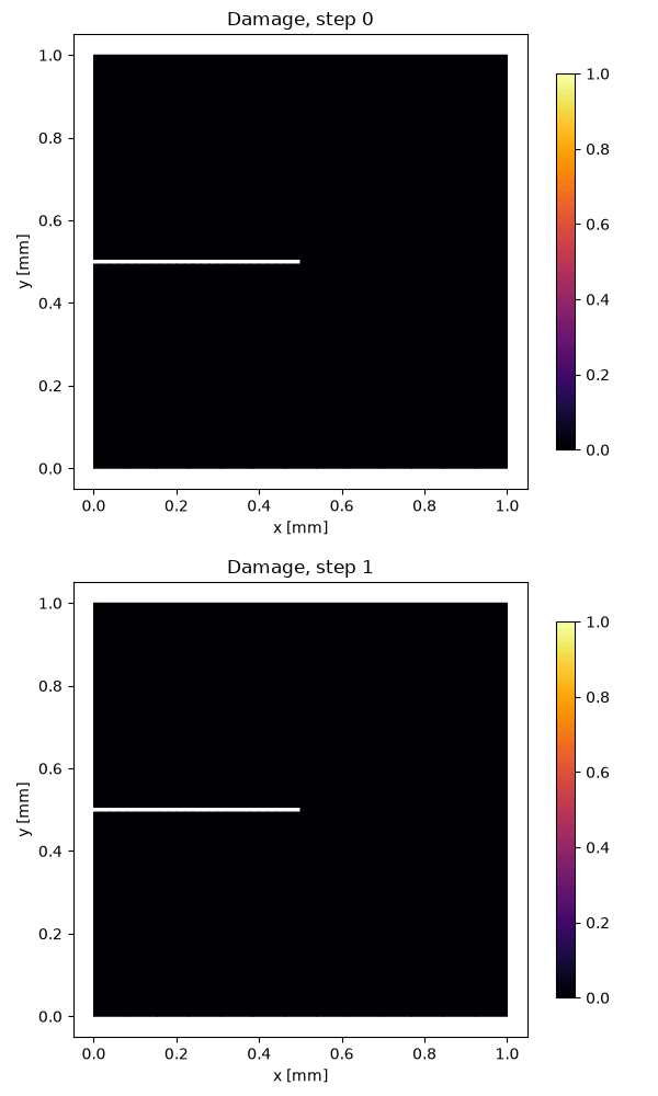
If the run generated damage_evolution.gif or damage_evolution.mp4, display it directly. For longer studies, prefer generating animations from the stored Zarr trajectory after the solve so rendering settings can be changed without rerunning the physics.

from IPython.display import Image, Video, display

gif_path = output_dir / "damage_evolution.gif"
mp4_path = output_dir / "damage_evolution.mp4"

if not gif_path.exists() and result.has_field("damage"):
    history_len = len(result.history("results")) if "results" in result.history_names() else num_steps
    frames = []
    for step_index in range(history_len):
        damage = np.nan_to_num(result.field("damage", step=step_index), nan=0.0, posinf=1.0, neginf=0.0)
        fig, ax = plt.subplots(figsize=(6, 5))
        im = ax.tripcolor(points[:, 0], points[:, 1], triangles, damage, shading="gouraud", cmap="inferno", vmin=0.0, vmax=1.0)
        ax.set_aspect("equal")
        ax.set_title(f"Damage, step {step_index}")
        ax.set_xlabel("x [mm]")
        ax.set_ylabel("y [mm]")
        fig.colorbar(im, ax=ax, shrink=0.82)
        fig.tight_layout()
        fig.canvas.draw()
        frames.append(np.asarray(fig.canvas.buffer_rgba())[:, :, :3].copy())
        plt.close(fig)
    PILImage.fromarray(frames[0]).save(
        gif_path, save_all=True,
        append_images=[PILImage.fromarray(frame) for frame in frames[1:]],
        duration=800, loop=0,
    )

if gif_path.exists():
    display(Image(filename=str(gif_path)))
elif mp4_path.exists():
    display(Video(str(mp4_path), embed=True))
else:
    print("No damage animation could be generated because the damage trajectory is not available.")

../_images/48bd99f4dd9933dac21b14c491a6dd2574a6e83ceeb637f0581ad2cd722a9d2a.gif

16. What to change for a real study¶

Start from a public example closest to your target physics.
Keep the .geo, .msh, config.yaml, run_fluent.py, setup preview, final field images, animations, and CSV histories together.
Use a mesh size that resolves the phase-field length scale; a common starting point is several elements across l0 near the crack path.
Validate the YAML with python -m phast run config.yaml --validate-only before using HPC time.
For dynamic fracture, switch the step and solver to explicit, include density, and verify the stable time step.
For quasi-static fracture, monitor staggered convergence and load-displacement response before trusting crack paths.
Archive the result directory, not only the notebook. The result directory is the reproducible simulation artifact.

17. Controlled exercises and exit questions¶

Change only one quantity per run and use a new output directory.

Exercise A: mesh size¶

Before changing h_bulk, predict the direction of change in element count, memory use, and runtime. Regenerate the mesh, inspect the actual counts, and explain whether the observation agrees with the prediction. This is a software and discretization exercise, not a convergence claim.

Exercise B: phase-field length scale¶

Change l0 while keeping the mesh fixed. Calculate h_bulk/l0 and explain why interpreting a damage profile becomes unsafe when the regularized field is poorly resolved. Do not compare apparent crack paths as scientific evidence from this two-step workflow.

Exercise C: loading¶

Change u_top while keeping the number of steps fixed. Predict how the increment size changes and identify which history should reveal the mechanical response.

Exit questions¶

What physical decision is represented by each named mesh region?
What did --validate-only establish, and what did it leave untested?
Which files identify the executed solver route and repository revision?
What additional mesh, convergence, calibration, and comparison evidence would be required before reporting a fracture result?

If execution was unavailable, answer using the rendered outputs, then inspect the retained-results notebook. Continue with From a tutorial to a first research study before adapting the example to a research problem.