Understanding a layered DCB simulation with PhAST¶

Physical question: how does a crack opening along a weak bulk layer interact with a circular region that is harder to fracture?

A double-cantilever-beam (DCB) specimen opens in two arms above and below an initial crack. This DCB-style teaching model uses that loading idea. It is not an ASTM test reproduction or an experimentally calibrated specimen.

By completing this notebook, you will be able to:

• identify geometry, mesh, material regions, the initial crack, and boundary conditions;

• connect displacement, strain, stress, and phase-field damage to their physical meanings;

• explain the implicit staggered solution used in this quasi-static example;

• edit a copy of the standard YAML and submit it through the normal PhAST commands;

• distinguish prescribed initial damage from computed crack growth;

• interpret images, an animation, response histories, and a controlled material comparison.

Default mode: inspect the checked-in results without rerunning the fracture simulation. The optional full solve is disabled by RUN_NEW_SIMULATION = False. The retained fine calculation took about 968 seconds on its recorded CPU run; this is not a runtime estimate for your computer.

Scope: two-dimensional, small-strain, plane-stress, quasi-static Amor AT2 fracture on a structured triangular mesh. The three regions are bulk materials. A weak layer is not an independent cohesive or interphase-debonding law. The retained results do not establish penetration, completed bypass, mesh independence, or physical validation.

This notebook uses the existing PhAST configuration, CLI, result reader, and comparison script. It does not implement another FEM solver.

1. Install and open the notebook¶

Use Python 3.10 or newer. Python 3.11 is a suitable choice for a teaching environment. This multi-material route uses CPU calculations in double precision. A GPU, a separate PhAST C++ compilation, and optional external solver packages are not required for this example.

Clone the complete repository, not only this notebook: the example configuration and retained figures are required inputs. Start Jupyter from the repository root and select the Python (PhAST) kernel.

macOS or Linux¶

# Clone the source, including example inputs and retained results.
git clone https://github.com/CEMS-Lab/PhAST.git
cd PhAST

# Use an installed Python >=3.10 to create an isolated environment.
python3 -m venv .venv
source .venv/bin/activate

# Install PhAST and Jupyter into that same environment.
python -m pip install --upgrade pip
python -m pip install -e .
python -m pip install jupyterlab ipykernel
python -m ipykernel install --user --name phast --display-name "Python (PhAST)"

# Open the explainer.
python -m jupyter lab docs/tutorial/notebook_layered_dcb.ipynb

Windows PowerShell¶

# Clone the same source.
git clone https://github.com/CEMS-Lab/PhAST.git
cd PhAST

# The selected Python 3 installation must be version 3.10 or newer.
py -3 -m venv .venv

# Calling the environment's Python directly avoids activation-policy issues.
.\.venv\Scripts\python.exe -m pip install --upgrade pip
.\.venv\Scripts\python.exe -m pip install -e .
.\.venv\Scripts\python.exe -m pip install jupyterlab ipykernel
.\.venv\Scripts\python.exe -m ipykernel install --user --name phast --display-name "Python (PhAST)"
.\.venv\Scripts\python.exe -m jupyter lab docs/tutorial/notebook_layered_dcb.ipynb

The base installation supplies the solver and plotting dependencies. The optional python -m pip install -r requirements.txt route follows the repository dependency list. Consult Installation for platform-specific and optional backend requirements.

Already installed? Do not clone again. Open this notebook from the checkout you installed. Run cells from top to bottom. After changing the parameter cell, restart the kernel and run all cells so that the schematic, configuration, and output paths remain consistent.

# Configuration, plotting, and calls to PhAST; no replacement FEM implementation.
from __future__ import annotations

import copy
import csv
import json
import math
import os
from pathlib import Path
import platform
import subprocess
import sys
import uuid

if sys.version_info < (3, 10):
    raise RuntimeError("Select a notebook kernel with Python 3.10 or newer.")

import matplotlib.pyplot as plt
from matplotlib.patches import Circle, Rectangle
import numpy as np
import yaml
from IPython.display import Image, Markdown, display
import phast

# Set this only if automatic discovery cannot locate your cloned repository.
REPOSITORY_PATH: str | None = None


def find_repository(override: str | None) -> Path:
    if override is not None:
        candidates = [Path(override).expanduser().resolve()]
    else:
        current = Path.cwd().resolve()
        package = Path(phast.__file__).resolve()
        candidates = [current, *current.parents, *package.parents]
    for candidate in candidates:
        if (candidate / "examples/two_material_dcb/config.yaml").is_file():
            return candidate
    raise FileNotFoundError(
        "Clone the complete PhAST repository and, if necessary, "
        "set REPOSITORY_PATH to that checkout."
    )


ROOT = find_repository(REPOSITORY_PATH)
if not Path(phast.__file__).resolve().is_relative_to((ROOT / "src/phast").resolve()):
    raise RuntimeError(
        "The selected kernel imports a different PhAST installation. "
        "Install this checkout with python -m pip install -e . and restart the kernel."
    )

EXAMPLE = ROOT / "examples/two_material_dcb"
RETAINED = EXAMPLE / "results"
REFERENCE_CONFIG = EXAMPLE / "config.yaml"
reference_config = yaml.safe_load(REFERENCE_CONFIG.read_text(encoding="utf-8"))
config = copy.deepcopy(reference_config)  # Keep the checked-in reference unchanged.

plt.style.use("default")
plt.rcParams.update({"figure.facecolor": "white", "axes.facecolor": "white"})
print("Python:", platform.python_version())
print("PhAST:", getattr(phast, "__version__", "version not exposed"))
print("Repository:", ROOT)
print("Reference input:", REFERENCE_CONFIG.relative_to(ROOT))

Python: 3.11.18
PhAST: version not exposed
Repository: /home/runner/work/PhAST/PhAST
Reference input: examples/two_material_dcb/config.yaml

2. State the physical problem¶

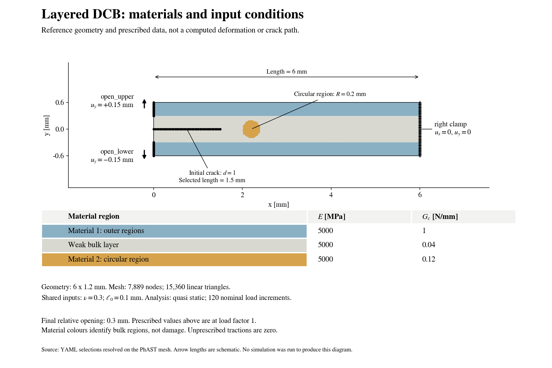
Blue identifies the outer Material 1, grey the weak bulk layer, and ochre the circular Material 2. This is a reference input diagram, not a new simulation result. The diagram and the editable schematic below use the same colours; red remains reserved for damage. The final prescribed displacements are \(+0.15\) mm and \(-0.15\) mm, giving a relative opening of \(0.30\) mm.

The reference rectangle is 6.0 mm long and 1.2 mm high. A weak bulk layer occupies its central 0.6 mm. A circular region of radius 0.20 mm is centred at \((2.2,0)\) mm inside that layer. An initial damaged line extends from the left edge to \(x=1.5\) mm.

The right edge is fixed. Opposite vertical displacements open the upper and lower portions of the left edge. The final values are \(+0.15\) mm above and \(-0.15\) mm below: 0.30 mm total opening.

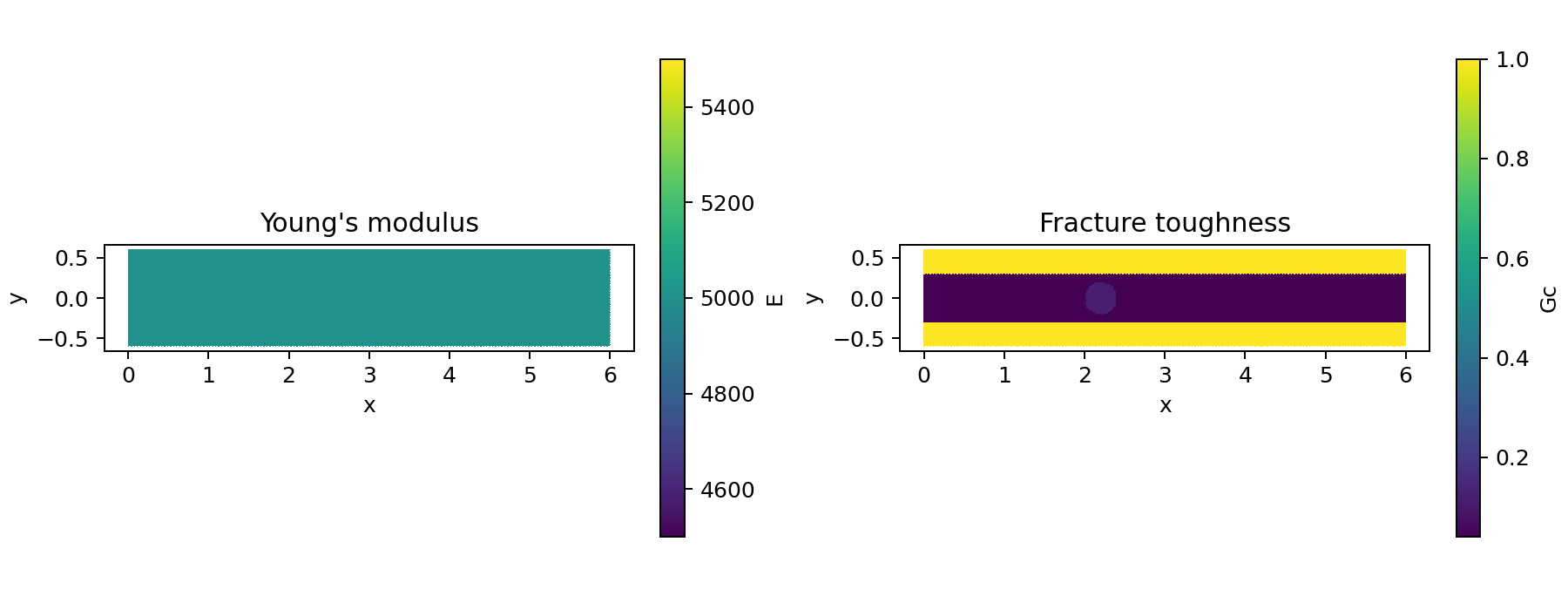
The elastic stiffness is initially identical in all three regions. The circle is therefore tougher, not stiffer, than the weak layer. This is a three-region model despite the example directory’s historical name.

Before viewing the result: sketch two possible crack paths. Would a larger \(G_c\) necessarily force a crack around the circle? Keep your prediction separate from what the computed fields show.

3. Edit the study parameters in one place¶

The defaults below reproduce the declared fine-reference input values. They do not guarantee bit-identical reproduction of a historical run: its exact generating source revision was not recorded.

Students normally edit this cell. The following cells map these variables into the existing schema-2 configuration, rather than requiring a new simulation program.

Units: lengths and displacements are in mm, \(E\) is in MPa (\(\mathrm{N/mm^2}\)), and \(G_c\) is in N/mm. Poisson’s ratio \(\nu\) and damage \(d\) are dimensionless. The regularisation length \(\ell_0\) is a model parameter, not the mesh spacing. Density does not enter this quasi-static equilibrium calculation.

# Enable only when you intend to run the full fracture calculation.
RUN_NEW_SIMULATION = False

# Geometry and mesh. An even ny places nodes on the midline y = 0.
L = 6.0                 # Length [mm].
H = 1.2                 # Height [mm].
layer_height = 0.60     # Weak bulk-layer thickness [mm].
circle_x = 2.20         # Material 2 centre [mm].
circle_y = 0.0
circle_radius = 0.20    # Material 2 radius [mm].
initial_crack_length = 1.50
crack_selection_width = 0.012  # Selection distance [mm], not crack opening.
nx = 160                # Cells along x; each cell is split into two T3 triangles.
ny = 48

# Material parameters. YAML uses Gc for G_c and l0 for ell_0.
E = 5000.0              # Outer-material and weak-layer Young's modulus [MPa].
E_material_2 = 5000.0   # Keep equal to E to isolate the toughness contrast.
nu = 0.30
G_c_outer = 1.00        # Outer material fracture resistance [N/mm].
G_c_layer = 0.04        # Weak-layer fracture resistance [N/mm].
G_c_material_2 = 0.12   # Circular-region fracture resistance [N/mm].
ell_0 = 0.10           # Shared regularisation length [mm].
eta = 1.0e-6           # Shared residual stiffness parameter, dimensionless.

# This is a load sequence, not a duration in seconds.
final_opening = 0.30    # Total separation of the loaded arms [mm].
number_of_load_levels = 121  # Includes zero: 120 nominal nonzero increments.

4. Geometry, mesh, and named regions¶

Geometry specifies the physical dimensions. Meshing divides the domain into finite elements. A T3 element is a three-node triangle with linear interpolation of the nodal fields.

PhAST constructs this mesh using geometry.type: structured_rectangle. This example does not require a separate geometry file. Named regions select material elements, the starter crack, and boundary nodes.

The next cell keeps the circle and its complementary selections consistent. It updates the layer rectangles and load bounds when dimensions change. The right clamp uses side: right and therefore follows the right edge.

Material assignment uses triangle centroids. The circle is approximated by selected triangles; its boundary is not a curved, conforming mesh.

# Geometry and mesh are specified through PhAST's standard configuration.
config["geometry"]["parameters"].update(
    length=L, height=H, origin=[0.0, -H / 2.0], nx=nx, ny=ny
)
regions = config["regions"]

# Keep the disk and both complementary outside-circle selectors identical.
for selector in (
    regions["material_2_region"],
    regions["material_1_region"]["selectors"][0],
    regions["weak_midline_region"]["selectors"][1],
):
    selector.update(center=[circle_x, circle_y], radius=circle_radius)

# Update the weak-layer rectangle and the rectangle used by its complement.
for rectangle in (
    regions["weak_midline_region"]["selectors"][0],
    regions["material_1_region"]["selectors"][1]["selector"],
):
    rectangle.update(origin=[0.0, -layer_height / 2.0], size=[L, layer_height])

# Starter crack and exterior boundary selections.
regions["initial_crack"].update({
    "from": [0.0, 0.0], "to": [initial_crack_length, 0.0],
    "thickness": crack_selection_width,
})
regions["right_clamp"] = {
    "kind": "node_region", "type": "boundary", "side": "right", "tolerance": 1.0e-8,
}
regions["upper_load"].update(
    axis="x", value=0.0, bounds={"y": [layer_height / 2.0, H / 2.0]}
)
regions["lower_load"].update(
    axis="x", value=0.0, bounds={"y": [-H / 2.0, -layer_height / 2.0]}
)

# Here h is the maximum triangle-edge length, not an equivalent-area diameter.
h = math.hypot(L / nx, H / ny)
print(f"Expected mesh: {(nx + 1) * (ny + 1):,} nodes, {2 * nx * ny:,} triangles")
print(f"Maximum triangle edge h = {h:.5f} mm; h / ell_0 = {h / ell_0:.3f}")
print("These sizes follow from the input; they are not completed simulation results.")

Expected mesh: 7,889 nodes, 15,360 triangles
Maximum triangle edge h = 0.04507 mm; h / ell_0 = 0.451
These sizes follow from the input; they are not completed simulation results.

For the reference mesh, \(h\approx0.0451\) mm and \(h/\ell_0\approx0.451\). The often-used criterion \(h\leq\ell_0/2\) concerns resolution of the regularised crack. It does not establish mesh-independent forces, crack trajectories, or physical accuracy.

Refining nx and ny at fixed \(\ell_0\) examines discretisation effects. Changing \(\ell_0\) changes the model as well as its resolution requirements. These are different experiments.

5. Materials and the phase-field variable¶

Displacement \(\mathbf u\) describes movement. Strain \(\boldsymbol\varepsilon\) describes local deformation. Stress \(\boldsymbol\sigma\) describes internal force per area. The scalar phase field \(d\) describes damage: \(d=0\) is intact and \(d=1\) is fully damaged in this convention.

For small strain,

The reference model degrades the selected crack-driving elastic energy using

The small positive \(\eta\) avoids exactly zero residual stiffness. It is not a fourth material phase.

A useful energy description, per unit out-of-plane thickness, is

Here \(\Omega\) is the specimen domain, \(\psi_0^+\) is the elastic energy selected to drive damage, \(\psi_0^-\) is the retained part, and \(W_{\mathrm{ext}}\) is external work. The AT2 crack term spreads damage over a length controlled by \(\ell_0\).

This input uses the Amor volumetric-deviatoric energy split. It is not a Miehe spectral split. The multi-material adapter does not support arbitrary replacement of the split or fracture law.

The implementation uses a history field to retain the maximum previous crack-driving energy. That update is distinguished from unconstrained minimisation of the displayed instantaneous energy.

# Preserve the existing material definitions and assignment list.
for name, youngs_modulus, fracture_resistance in (
    ("material_1", E, G_c_outer),
    ("weak_midline", E, G_c_layer),
    ("material_2", E_material_2, G_c_material_2),
):
    parameters = config["materials"][name]["parameters"]
    parameters.update(
        E=youngs_modulus, nu=nu, Gc=fracture_resistance, l0=ell_0,
        eta_residual=eta, energy_split="amor", pf_model="AT2", plane_stress=True,
    )
    print(f"{name:15s}: E = {youngs_modulus:g} MPa, Gc = {fracture_resistance:g} N/mm")

print("\nAssignments are unchanged:")
print(yaml.safe_dump(config["assignments"], sort_keys=False))

material_1     : E = 5000 MPa, Gc = 1 N/mm
weak_midline   : E = 5000 MPa, Gc = 0.04 N/mm
material_2     : E = 5000 MPa, Gc = 0.12 N/mm

Assignments are unchanged:
- material: material_1
  region: material_1_region
- material: weak_midline
  region: weak_midline_region
- material: material_2
  region: material_2_region

6. Initial crack, restraints, and opening displacements¶

The initial crack is a selected row of nodes with maintained damage \(d=1\). This defines the starting defect. It does not prescribe the later path around or through Material 2.

The load factor \(s\) increases from zero to one. The final prescribed opening is \(\Delta\). Other exterior boundary segments have the natural zero-traction condition where no displacement is prescribed. The vertical loading conditions do not fix horizontal motion on the left segments.

# Keep the condition types, names, and active-condition list from the reference.
config["initial_conditions"][0]["value"] = 1.0
for boundary in config["boundary_conditions"]:
    if boundary["name"] == "open_upper":
        boundary["value"] = final_opening / 2.0
    elif boundary["name"] == "open_lower":
        boundary["value"] = -final_opening / 2.0

print(yaml.safe_dump(config["boundary_conditions"], sort_keys=False))

- name: clamp_x
  type: fix
  region: right_clamp
  dof: x
- name: clamp_y
  type: fix
  region: right_clamp
  dof: y
- name: open_upper
  type: prescribe
  region: upper_load
  dof: y
  value: 0.15
- name: open_lower
  type: prescribe
  region: lower_load
  dof: y
  value: -0.15

# Input schematic only. PhAST, not this drawing, constructs the actual FEM mesh.
figure, axis = plt.subplots(figsize=(11, 3.5), constrained_layout=True)
axis.add_patch(Rectangle((0.0, -H / 2.0), L, H, facecolor="#8AB0C4", edgecolor="0.25", label="Material 1: outer regions"))
axis.add_patch(Rectangle(
    (0.0, -layer_height / 2.0), L, layer_height,
    facecolor="#D8D8D1", edgecolor="0.45", label="Weak bulk layer",
))
axis.add_patch(Circle(
    (circle_x, circle_y), circle_radius,
    facecolor="#D6A24B", edgecolor="0.15", label="Material 2",
))
axis.plot([0.0, initial_crack_length], [0.0, 0.0],
          color="black", linewidth=3, label="Prescribed starter crack")
axis.plot([L, L], [-H / 2.0, H / 2.0],
          color="black", linewidth=4, label="Fixed right edge")
load_y = (H + layer_height) / 4.0
for sign, label in ((1.0, "+ opening"), (-1.0, "- opening")):
    axis.annotate(
        "", xy=(0.0, sign * (load_y + 0.12 * H)), xytext=(0.0, sign * load_y),
        arrowprops={"arrowstyle": "->", "color": "0.15", "lw": 1.8},
    )
    axis.text(-0.08 * L, sign * load_y, label, ha="right", va="center", fontsize=9)
axis.set(
    xlim=(-0.30 * L, 1.03 * L), ylim=(-0.8 * H, 0.8 * H),
    xlabel="x [mm]", ylabel="y [mm]",
    title="Edited input: geometry and boundary-condition schematic",
)
axis.set_aspect("equal")
axis.legend(loc="upper center", bbox_to_anchor=(0.5, -0.28), ncol=2, frameon=False)
plt.show()

7. What does the staggered solver do?¶

Quasi-static means inertia is omitted: each accepted load level seeks mechanical equilibrium. It does not mean explicit time stepping with a small time step. The load factor is not elapsed physical time.

At one load level, PhAST alternates between two subproblems:

1. Hold damage fixed and solve mechanical equilibrium for displacement. With no body force, the strong balance is \(\nabla\!\cdot\boldsymbol\sigma=\mathbf0\).

2. Evaluate strain and the crack-driving elastic energy. Update the history \(\mathcal H_n=\max(\mathcal H_{n-1},\psi_0^+(\boldsymbol\varepsilon_n))\).

3. Hold that driving field fixed and solve the spatial damage problem subject to bounds and maintained damage conditions.

4. Recompute the coupled state until the configured subproblem and staggered criteria are met. Otherwise, the run may reduce the load increment or stop.

An implicit subproblem determines the unknown current field by satisfying equations or constrained optimality conditions. It does not add a prescribed damage increment at every node. Both mechanics and damage are implicit here. Explicit mechanics in a dynamic example is a different route, not a supported option of this multi-material DCB adapter.

Why is AT2 damage often called linear?¶

For fixed \(\mathcal H\) and material coefficients, the unconstrained weak damage equation is

The test function \(q\) represents an admissible variation of damage. With finite-element shape functions \(N_i\), interpolation gives \(A\mathbf d=\mathbf b\), where

Quadratic degradation gives a linear unconstrained subproblem when the driving field is fixed. It does not make the complete fracture calculation linear. Bounds \(d_{\mathrm{previous}}\leq d\leq1\), prescribed damage, spatial coupling, iterative linear algebra, and repeated staggered updates still require work.

The projected residual measures the constrained damage problem, rather than requiring the unconstrained residual to vanish at every active bound. The matrix notation above explains the problem; this notebook delegates its implementation to PhAST instead of assembling a second FEM system.

# Load levels and solver iterations are different quantities.
step = config["analysis_steps"][0]
step["controls"]["number_of_steps"] = number_of_load_levels

# Keep the supported route and the reference convergence controls.
# Changing this string alone does not enable dynamic multi-material fracture.
config["solver"]["type"] = "quasi_static"
print("Analysis:", step["type"])
print("Nominal nonzero increments:", number_of_load_levels - 1)
print("\nNumerical controls inherited from the reference:")
print(yaml.safe_dump(config["solver"], sort_keys=False))

Analysis: quasi_static
Nominal nonzero increments: 120

Numerical controls inherited from the reference:
type: quasi_static
mechanics_backend: auto
mechanics_tolerance: 1.0e-09
mechanics_relative_tolerance: 1.0e-08
mechanics_max_iterations: 30
damage_tolerance: 1.0e-08
damage_max_iterations: 500
damage_bounds_method: projected_cg
maximum_staggered_iterations: 500
staggered_damage_tolerance: 1.0e-05
projected_residual_tolerance: 1.0e-05
damage_relaxation: 0.7
automatic_cutback: true
minimum_load_increment: 0.00025
maximum_cutbacks: 40
crack_front_threshold: 0.8

The fine reference accepts 120 nonzero increments. With cutbacks, a run can accept more increments than the nominal count. Solver iteration limits count attempts to solve a subproblem, not additional physical load levels.

Automatic cutback is not evidence of success by itself. Inspect accepted-step residuals and final status. Increasing an iteration limit or loosening a tolerance does not establish physical accuracy. This route reports its selected mechanics backend during execution; the requested value auto alone does not identify that backend.

8. Save one YAML and use the standard commands¶

The following cells write a new input under runs/ and leave the checked-in reference unchanged. Each notebook execution receives a new directory so results from different parameter choices are not mixed.

The command sequence is:

python -m phast explain-config CONFIG
python -m phast run CONFIG --validate-only
python -m phast run CONFIG --output_dir RUN

Here CONFIG and RUN are placeholders. The code below supplies actual paths. Explanation describes the input without creating a mesh. Multi-material validation constructs the geometric mesh to check selections and assignments, but does not solve the FEM problem. Neither step establishes numerical convergence or physical validity.

# All new files are outside the curated example directory.
output_root = Path(os.environ.get("PHAST_NOTEBOOK_OUTPUT_ROOT", str(ROOT / "runs")))
STUDY_DIR = output_root / f"dcb_student_{uuid.uuid4().hex[:10]}"
STUDY_DIR.mkdir(parents=True, exist_ok=False)
CONFIG_PATH = STUDY_DIR / "config.yaml"
RUN_DIR = STUDY_DIR / "solution"

config["name"] = "Layered DCB student study"
config["outputs"]["directory"] = str(RUN_DIR.resolve())
for field in config["outputs"]["fields"]:
    if field["name"] == "trajectory":
        field.update(format="h5", every=1)
CONFIG_PATH.write_text(yaml.safe_dump(config, sort_keys=False), encoding="utf-8")
print("Student input:", CONFIG_PATH)
print("New result directory, if solving is enabled:", RUN_DIR)
print("The checked-in reference and retained results have not been modified.")

Student input: /home/runner/work/PhAST/PhAST/runs/dcb_student_276a3e8077/config.yaml
New result directory, if solving is enabled: /home/runner/work/PhAST/PhAST/runs/dcb_student_276a3e8077/solution
The checked-in reference and retained results have not been modified.

# Use the notebook kernel's Python rather than a different shell environment.
def run_cli(arguments: list[str]) -> None:
    completed = subprocess.run(
        [sys.executable, "-m", "phast", *arguments],
        cwd=ROOT, capture_output=True, text=True, check=False,
    )
    print(completed.stdout)
    if completed.stderr:
        print(completed.stderr)
    if completed.returncode != 0:
        raise RuntimeError("PhAST rejected the command. Read the first error above before proceeding.")


run_cli(["explain-config", str(CONFIG_PATH)])
run_cli(["run", str(CONFIG_PATH), "--validate-only"])

Config: /home/runner/work/PhAST/PhAST/runs/dcb_student_276a3e8077/config.yaml
Schema version: 2
Problem: Layered DCB student study
Reference: Qualitative confined-layer AT2 teaching model; not experimental calibration or a cohesive-interface model

Geometry and mesh
  type: structured_rectangle; units: mm
  length: 6.0
  height: 1.2
  origin: [0.0, -0.6]
  nx: 160
  ny: 48

Regions (declared selections, not resolved node/element sets)
  material_1_region: element_region; {'type': 'all_of', 'selectors': [{'type': 'outside_circle', 'center': [2.2, 0.0], 'radius': 0.2}, {'type': 'not', 'selector': {'type': 'rectangle', 'origin': [0.0, -0.3], 'size': [6.0, 0.6]}}]}
  weak_midline_region: element_region; {'type': 'all_of', 'selectors': [{'type': 'rectangle', 'origin': [0.0, -0.3], 'size': [6.0, 0.6]}, {'type': 'outside_circle', 'center': [2.2, 0.0], 'radius': 0.2}]}
  material_2_region: element_region; {'type': 'circle', 'center': [2.2, 0.0], 'radius': 0.2}
  initial_crack: node_region; {'type': 'line_segment', 'from': [0.0, 0.0], 'to': [1.5, 0.0], 'thickness': 0.012}
  right_clamp: node_region; {'type': 'boundary', 'side': 'right', 'tolerance': 1e-08}
  upper_load: node_region; {'type': 'boundary_segment', 'axis': 'x', 'value': 0.0, 'bounds': {'y': [0.3, 0.6]}, 'tolerance': 1e-08}
  lower_load: node_region; {'type': 'boundary_segment', 'axis': 'x', 'value': 0.0, 'bounds': {'y': [-0.6, -0.3]}, 'tolerance': 1e-08}

Materials and assignments
  material_1: phase_field; region=material_1_region
    E: 5000.0
    nu: 0.3
    Gc: 1.0
    l0: 0.1
    rho: 1.0
    eta_residual: 1e-06
    energy_split: amor
    pf_model: AT2
    plane_stress: True
  weak_midline: phase_field; region=weak_midline_region
    E: 5000.0
    nu: 0.3
    Gc: 0.04
    l0: 0.1
    rho: 1.0
    eta_residual: 1e-06
    energy_split: amor
    pf_model: AT2
    plane_stress: True
  material_2: phase_field; region=material_2_region
    E: 5000.0
    nu: 0.3
    Gc: 0.12
    l0: 0.1
    rho: 1.0
    eta_residual: 1e-06
    energy_split: amor
    pf_model: AT2
    plane_stress: True

Initial conditions
  damage: region=initial_crack; value=1.0

Boundary conditions
  clamp_x: fix; region=right_clamp; component=0; value=None
  clamp_y: fix; region=right_clamp; component=1; value=None
  open_upper: prescribe; region=upper_load; component=1; value=0.15
  open_lower: prescribe; region=lower_load; component=1; value=-0.15

Analysis steps
  opening: quasi_static; controls={'number_of_steps': 121}
    active boundary conditions: clamp_x, clamp_y, open_upper, open_lower

Solver (requested)
  type: quasi_static
  mechanics_backend: auto
  mechanics_tolerance: 1e-09
  mechanics_relative_tolerance: 1e-08
  mechanics_max_iterations: 30
  damage_tolerance: 1e-08
  damage_max_iterations: 500
  damage_bounds_method: projected_cg
  maximum_staggered_iterations: 500
  staggered_damage_tolerance: 1e-05
  projected_residual_tolerance: 1e-05
  damage_relaxation: 0.7
  automatic_cutback: True
  minimum_load_increment: 0.00025
  maximum_cutbacks: 40
  crack_front_threshold: 0.8

Outputs
  output_dir: /home/runner/work/PhAST/PhAST/runs/dcb_student_276a3e8077/solution
  field trajectory: every=1; {'format': 'h5'}
  field displacement: every=1; {}
  field strain: every=1; {}
  field stress: every=1; {}
  field damage: every=1; {}
  field vtu: every=1; {}
  history reaction_force: every=1; region=upper_load; component=1
  history max_damage: every=1; region=None; component=None
  history solver_telemetry: every=1; region=None; component=None
  history timing_per_step: every=1; region=None; component=None
  visual initial_conditions: {}
  visual plots: {}
  visual animation: {'field': 'damage'}

Scope
  Declared settings only: no mesh, solver, or output directory was created.
  This summary does not confirm execution support, convergence, or physical accuracy.
  Check the requested execution route with: python -m phast run "/home/runner/work/PhAST/PhAST/runs/dcb_student_276a3e8077/config.yaml" --validate-only
  Multi-material validation resolves the geometric mesh to check selections and assignments.

OK: /home/runner/work/PhAST/PhAST/runs/dcb_student_276a3e8077/config.yaml passes schema-v2 workflow contract validation.

9. Optional: execute your edited problem¶

With RUN_NEW_SIMULATION = False, the next cell does not start a simulation. It selects the separately retained reference results for the interpretation exercises.

To compute new results, set that parameter to True, restart the kernel, and run all cells. This full reference calculation is not a two-second installation check. PhAST prints accepted increments, opening, reaction, crack-front position, and a residual as the solve progresses. A separate log is also saved.

A failed solve raises an error here. Partial output must not be presented as a completed reference run. Use a new study directory when retrying; the trajectory writer does not silently overwrite an existing HDF5 file.

run_completed = False
if not RUN_NEW_SIMULATION:
    print("No new FEM simulation requested. Later result cells use the retained fine reference.")
else:
    if RUN_DIR.exists():
        raise FileExistsError("The result directory already exists. Restart and run all cells for a new study.")
    command = [
        sys.executable, "-m", "phast", "run", str(CONFIG_PATH), "--output_dir", str(RUN_DIR),
    ]
    log_path = STUDY_DIR / "solver.log"
    # Stream the existing runner's progress, without another solver loop.
    with log_path.open("w", encoding="utf-8") as log:
        with subprocess.Popen(
            command, cwd=ROOT, stdout=subprocess.PIPE,
            stderr=subprocess.STDOUT, text=True, bufsize=1,
        ) as process:
            if process.stdout is None:
                raise RuntimeError("The solver output stream was not available.")
            for line in process.stdout:
                print(line, end="", flush=True)
                log.write(line)
            return_code = process.wait()
    if return_code != 0:
        raise RuntimeError(f"The solve failed. Inspect {log_path}; partial output is not a converged run.")
    run_completed = True
    print("\nThe PhAST command completed. Inspect its status and residuals below.")

RESULT_DIR = RUN_DIR if run_completed else RETAINED
RESULT_LABEL = "New student calculation" if run_completed else "Retained fine-reference calculation"
print("Selected result:", RESULT_LABEL)

No new FEM simulation requested. Later result cells use the retained fine reference.
Selected result: Retained fine-reference calculation

10. Read a result before drawing a conclusion¶

A successful command and a visually plausible crack are different kinds of evidence. Inspect the recorded status, finite values, convergence measures, and the meaning of each observable.

The response table is history.csv. Its opening column is relative arm opening in mm. The two-dimensional reaction is interpreted per unit out-of-plane thickness, in N/mm for this unit system. Comparison with an experimental force in N requires a specimen thickness and an appropriate two-dimensional idealisation.

The initial crack already has \(d=1\). Therefore, maximum_damage = 1 alone says nothing about new crack growth.

def read_history(path: Path) -> dict[str, np.ndarray]:
    required = ("opening", "reaction_force", "connected_crack_front_x", "projected_damage_residual")
    with path.open("r", encoding="utf-8", newline="") as stream:
        rows = list(csv.DictReader(stream))
    if not rows:
        raise ValueError(f"No accepted steps were found in {path.name}.")
    history = {
        key: np.asarray([float(row[key]) for row in rows], dtype=float)
        for key in required
    }
    if not all(np.isfinite(values).all() for values in history.values()):
        raise ValueError("A selected history contains non-finite values. Investigate rather than hiding them.")
    return history


history = read_history(RESULT_DIR / "history.csv")
summary = json.loads((RESULT_DIR / "summary.json").read_text(encoding="utf-8"))
if not summary.get("all_steps_converged", False):
    raise RuntimeError("The selected run does not report convergence of all accepted steps.")

for key in (
    "n_nodes", "n_elements", "accepted_steps", "cutbacks", "final_opening",
    "final_reaction_force", "final_connected_crack_front_x", "maximum_projected_damage_residual",
):
    print(f"{key}: {summary[key]}")
print("These are recorded numerical results, not experimental validation.")

figure, axes = plt.subplots(1, 3, figsize=(13, 3.5), constrained_layout=True)
axes[0].plot(history["opening"], history["reaction_force"], color="0.20")
axes[0].set_ylabel("Opening reaction per unit thickness [N/mm]")
axes[1].step(history["opening"], history["connected_crack_front_x"], where="post", color="0.20")
axes[1].set_ylabel("Maximum seed-connected x at d >= 0.80 [mm]")
axes[2].plot(history["opening"], history["projected_damage_residual"], color="0.20")
result_input = config if run_completed else reference_config
axes[2].axhline(
    result_input["solver"]["projected_residual_tolerance"],
    color="0.45", linestyle="--", label="Configured projected-residual tolerance",
)
axes[2].set_ylabel("Projected damage residual [solver convention]")
axes[2].legend(fontsize=8, frameon=False)
for axis in axes:
    axis.set_xlabel("Opening [mm]")
    axis.grid(alpha=0.2)
figure.suptitle(RESULT_LABEL)
plt.show()

n_nodes: 7889
n_elements: 15360
accepted_steps: 120
cutbacks: 0
final_opening: 0.3
final_reaction_force: 0.6149522713694282
final_connected_crack_front_x: 2.0625
maximum_projected_damage_residual: 6.910926739149559e-06
These are recorded numerical results, not experimental validation.

Reading the retained fine-reference result¶

The retained fine calculation reports 120 accepted increments, no cutbacks, and 0.30 mm final opening. Its maximum recorded projected damage residual is about \(6.91\times10^{-6}\), below the configured \(10^{-5}\) criterion. These are recorded results, not a new solve by this notebook.

The seed-connected front reaches \(x=2.0625\) mm at threshold \(d\geq0.80\). This is the largest \(x\) coordinate connected to the starter crack through damaged mesh edges, not the crack’s arc length. Passing the circle’s leftmost \(x\) coordinate does not establish penetration: a branch can advance above or below it without entering the disk.

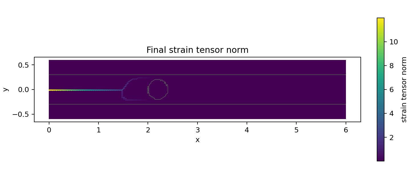
The retained field review found no seed-connected \(d\geq0.80\) node inside the tough disk. The images show branching near its flanks, not completed bypass. Both geometry and material contrast influence the result.

11. Displacement, strain, stress, and damage images¶

This section always shows the retained fine reference. The figures are not updated by editing the parameter cell. A separate cell below displays new images only after a fresh solve completes.

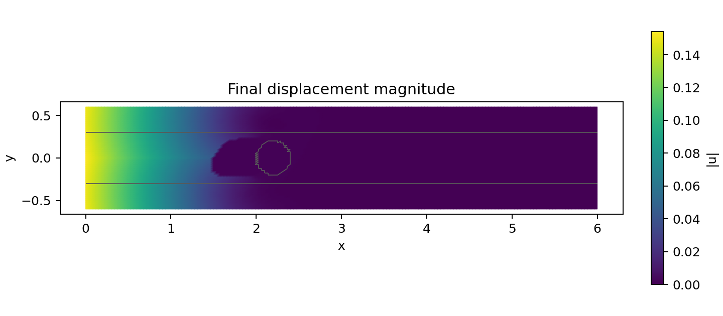
Displacement is motion in mm. Strain is dimensionless deformation. Stress components are in MPa. Damage is dimensionless. Read component names and any deformation scaling on each figure. Colour intensity is not comparable between different physical quantities.

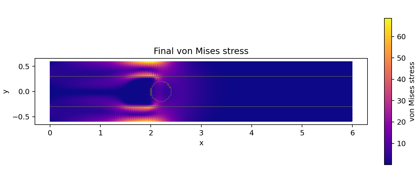
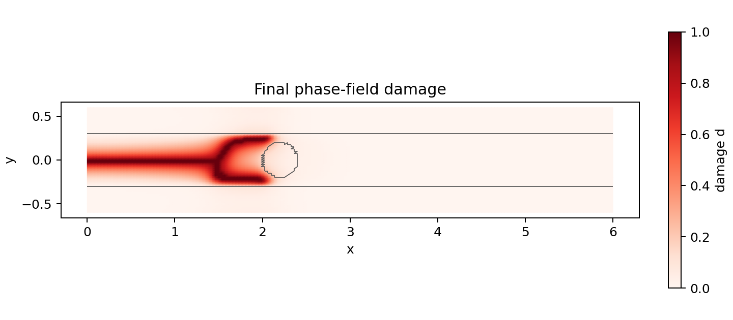
Follow the crack evolution¶

Identify the prescribed starter crack first, then newly damaged material. Grey outlines locate material boundaries; they are not additional crack constraints. This is a quasi-static load sequence, so animation speed is not physical crack speed.

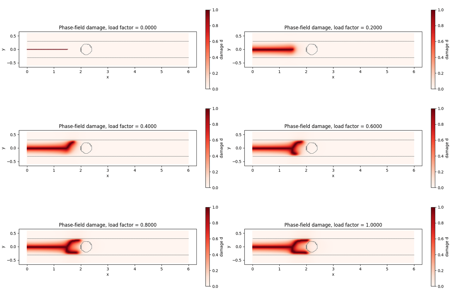
The final damage image is the static fallback if the animation does not play.

# New figures are generated by PhAST's existing example runner.
if run_completed:
    display(Markdown("### New student calculation: generated field images"))
    for filename in (
        "initial_conditions.png", "material_fields.png", "displacement_final.png",
        "strain_final.png", "stress_final.png", "damage_final.png", "damage_evolution.gif",
    ):
        display(Markdown(f"**{filename}**: new calculation, not the retained reference."))
        display(Image(filename=str(RUN_DIR / filename)))
else:
    print("No fresh-run figures exist for the edited input. The images above are the retained reference.")

No fresh-run figures exist for the edited input. The images above are the retained reference.

12. Inspect numerical fields through PhAST¶

A new run requests training_data.h5. It contains stored fields and mesh data and remains local, rather than being added to the public repository. The compact retained directory intentionally omits that full trajectory.

Use phast.load_result for a completed local run. Its field reader returns stored quantities; it does not infer raw fields from PNG images. A derived scalar such as von Mises stress requires the documented post-processing convention, especially for a two-dimensional model.

if run_completed:
    result = phast.load_result(RUN_DIR)
    print("Available stored fields:", result.field_names())
    for field_name in ("displacement", "strain", "stress", "damage"):
        values = np.asarray(result.field(field_name))  # Final stored step by default.
        if not np.isfinite(values).all():
            raise ValueError(f"Non-finite values in {field_name} require investigation.")
        print(field_name, "shape:", values.shape, "dtype:", values.dtype)
    damage = np.asarray(result.field("damage"))
    if damage.min() < -1.0e-8 or damage.max() > 1.0 + 1.0e-8:
        raise ValueError("The final damage field lies outside its expected numerical bounds.")
else:
    print("Raw fine-reference HDF5 fields are not part of the compact public results.")
    print("Run a new calculation before using this field-loading section.")

Raw fine-reference HDF5 fields are not part of the compact public results.
Run a new calculation before using this field-loading section.

13. What changes without the circle’s toughness contrast?¶

A useful comparison changes one physical input while holding the other choices fixed. Two complete existing inputs are available:

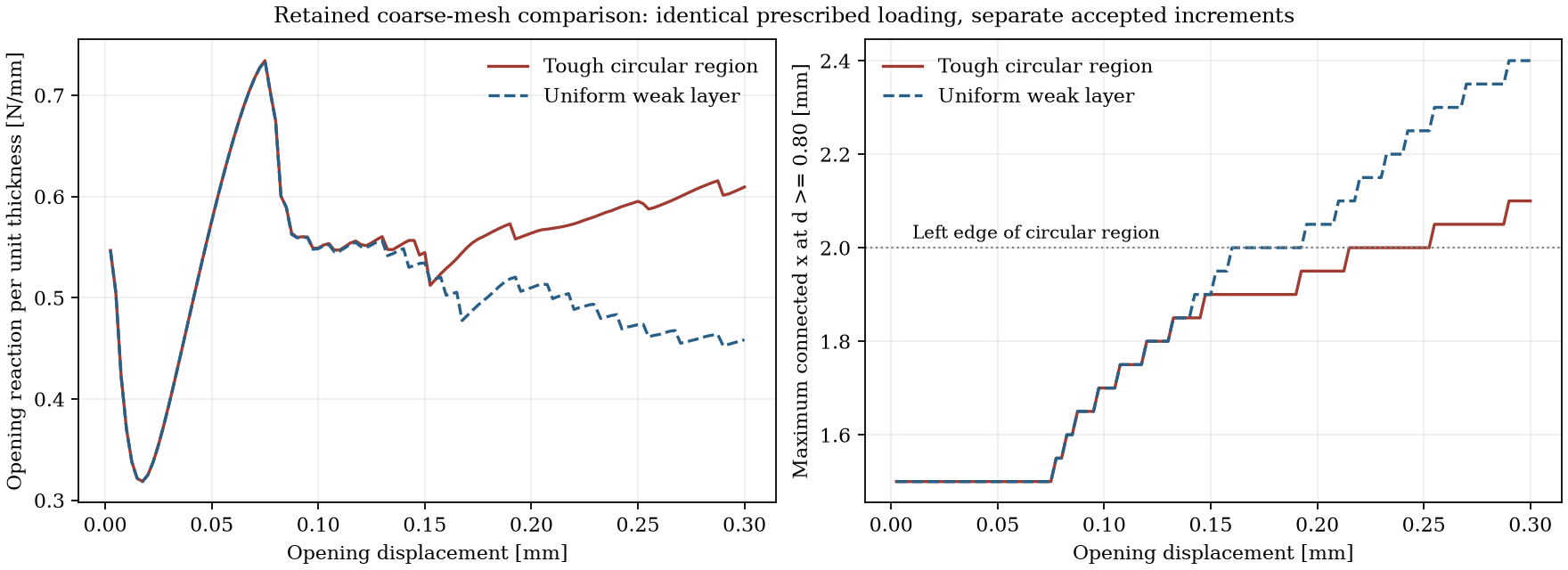
• examples/two_material_dcb/comparisons/tough_region.yaml: disk \(G_c=0.12\) N/mm;

• examples/two_material_dcb/comparisons/uniform_layer.yaml: disk \(G_c=0.04\) N/mm, equal to the weak layer.

Both use a separate coarse \(120\times48\) mesh, not the fine grid above. Outer material remains fracture-resistant: the control is a uniform weak layer, not a homogeneous specimen. Elastic properties and prescribed loading are held fixed.

At 0.30 mm opening, the retained tough-region case has about 0.60938 N/mm reaction and a connected front at 2.10 mm. The control has about 0.45847 N/mm and a front at 2.40 mm. Both cases branch. The circle cannot therefore be identified as the sole cause of branching.

The control required three cutbacks and has different accepted openings. Compare each history against its own opening coordinate, not by subtracting corresponding CSV rows. The next command only replots retained data. It does not run either solver or use your edited input.

# Reuse the checked-in comparison script and its provenance/checksum checks.
comparison_directory = STUDY_DIR / "retained_comparison"
comparison = subprocess.run(
    [
        sys.executable, str(EXAMPLE / "compare_results.py"),
        "--output-dir", str(comparison_directory),
    ],
    cwd=ROOT, capture_output=True, text=True, check=False,
)
print(comparison.stdout)
if comparison.returncode != 0:
    raise RuntimeError(comparison.stderr or "The retained comparison could not be replotted.")
for filename in ("matched_control_comparison.png", "matched_control_damage.png"):
    display(Markdown("**Retained coarse comparison. Not a new calculation of the edited problem.**"))
    display(Image(filename=str(comparison_directory / filename)))

Replotted retained data in /home/runner/work/PhAST/PhAST/runs/dcb_student_276a3e8077/retained_comparison
These figures show a qualitative confined-layer comparison. They do not establish penetration, completed bypass, or physical validation.

Retained coarse comparison. Not a new calculation of the edited problem.

Retained coarse comparison. Not a new calculation of the edited problem.

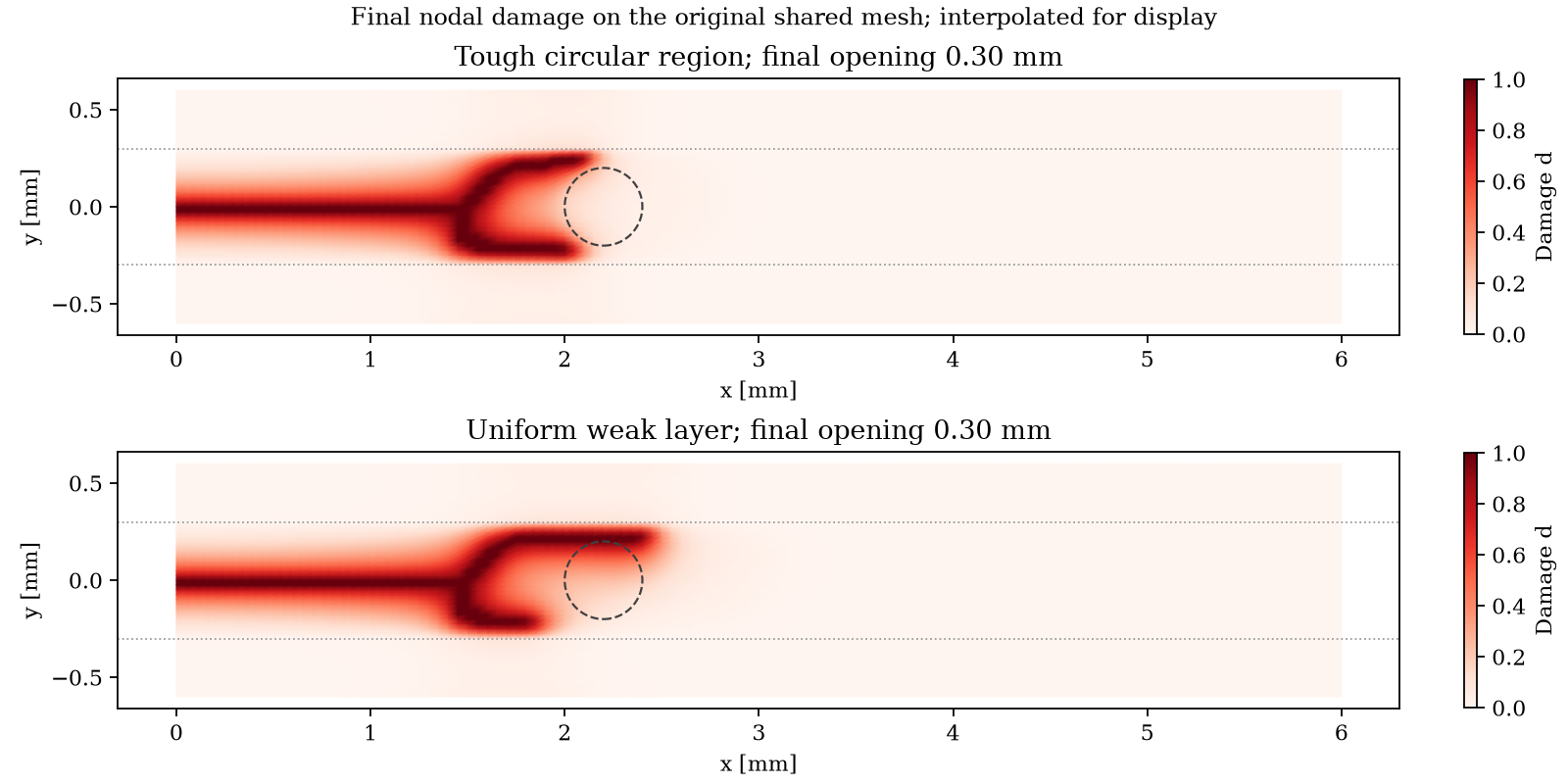
The comparison retains the original triangle connectivity. The coarse tough-region run did not write HDF5; the uniform-layer control did, and its stored mesh supplied that connectivity. Both new comparison inputs request HDF5 for local reruns. Exact historical generating-source identity remains unattested, as recorded in results/comparison_provenance.json.

To compute new coarse comparisons, submit each existing YAML through the same explain/check/run sequence, with distinct output directories. Do not compare a newly edited fine run directly with a retained coarse result and attribute the difference solely to material properties.

14. Guided student experiments¶

Predict an outcome first. Afterwards, record the input, source version, solver status, mesh measure, and result directory.

For a short laboratory session, interpret the retained results first. Plan long solves separately instead of making participants wait for a full fracture calculation before understanding the model.

Questions for a short written explanation¶

1. Why does the reference isolate a toughness contrast rather than a stiffness contrast inside the layer?

2. Why does \(\max d=1\) not establish crack growth?

3. What is fixed when the damage subproblem is described as linear?

4. Why can 121 nominal load levels lead to more than 120 accepted increments?

5. Why is a weak finite-width bulk layer not a cohesive interface law?

6. Which independent data would be needed before calling this an experimentally validated specimen model?

15. Troubleshooting and limits¶

This example does not establish a general interface, plasticity, three-dimensional composite, or dynamic multi-material workflow. Check the capability matrix before selecting another route.

The small-strain assumption, diffuse crack length relative to the circular region, elementwise boundary approximation, and confinement by the outer material affect interpretation. A convincing animation alone does not settle those modelling questions.

Ask for help and contribute¶

If an installation, configuration, execution, or interpretation step is unclear, open a GitHub issue. Include the YAML, command, operating system, Python and PhAST versions, source revision if known, and complete first error or solver log. State whether you inspected retained data or ran a new calculation.

Students, developers, and researchers are welcome to report unclear wording, propose a controlled comparison, review a result, or contribute a documented improvement. No familiarity with solver internals is required to ask a question.

See One configuration workflow for student simulations for the common input convention. The DCB example on GitHub contains the full configuration, result README, and evidence limitations.