From geometry to crack propagation: a square-plate SENT simulation
This tutorial performs a fresh phase-field fracture calculation with PhAST in the conventional finite-element order:
install and verify the software;
load the geometry;
generate and inspect the mesh and named boundaries;
define the material and phase-field model;
apply loads and boundary conditions;
select a supported analysis and solver route;
run the coupled problem with visible progress; and
inspect displacement, strain, stress, and damage and animate crack growth.
The model is the 40 mm by 40 mm B3 single-edge-notched tension (SENT) plate. A V-notch extends from the left boundary to (x=20) mm. This is a compact teaching calculation derived from the public B3 input, not a new benchmark validation or a mesh/time-step convergence study.
The calculation uses a CPU; no GPU is required. Installation, meshing, solving, and rendering have separate costs, and no portable runtime is claimed.
The B3 input retains its schema-v1 compatibility format to preserve the matched public example. For the single saved schema-v2 configuration workflow, use the standard problem-setup walkthrough. This notebook does not extend the schema-v2 solver capability boundary.
0. Install PhAST by the portable source route
Use Python >=3.10 with compatible dependency wheels. For a new source checkout:
git clone https://github.com/CEMS-Lab/PhAST.git
cd PhAST
python3 -m venv .venv
source .venv/bin/activate
python -m pip install --upgrade pip
python -m pip install -e . jupyterlab
python tools/run_sanitizer.py
python -m phast doctor
jupyter lab docs/tutorial/notebook_square_plate_fracture.ipynb
On Windows PowerShell, activate with .venv\Scripts\Activate.ps1.
Conda and Docker routes are in the installation guide. The base
CPU installation is sufficient; optional HPC backends are not required.
For an existing checkout or a documentation build, use that checkout and its
prepared environment. Do not clone or install an older release over it. The
clone command above selects public main, which is mutable; local changes
are not assumed to be published there.
from __future__ import annotations
import copy
import os
from pathlib import Path
import re
import shutil
import subprocess
import sys

from IPython.display import HTML, Image, Markdown, display
import matplotlib.pyplot as plt
import matplotlib.tri as mtri
from matplotlib.animation import FuncAnimation, PillowWriter
import numpy as np
import yaml


def find_repository_root(start: Path) -> Path:
    # Locate a source checkout from the notebook working directory.
    start = start.resolve()
    for candidate in (start, *start.parents):
        if (candidate / "pyproject.toml").is_file() and (candidate / "examples").is_dir():
            return candidate
    raise RuntimeError(
        "Run this notebook from a cloned PhAST repository. "
        "See the installation commands above."
    )

ROOT = find_repository_root(Path.cwd())
os.chdir(ROOT)
sys.path.insert(0, str(ROOT / "src"))
os.environ["PYTHONPATH"] = str(ROOT / "src") + os.pathsep + os.environ.get("PYTHONPATH", "")

import phast
from phast.core.mesh import FEMMesh
from phast.physics.material import Material

plt.rcParams.update({"font.family": "STIXGeneral", "mathtext.fontset": "stix"})

def require_finite(values, name):
    """Reject empty or non-finite data rather than disguising a failed solve."""
    array = np.asarray(values)
    if array.size == 0 or not np.isfinite(array).all():
        raise ValueError(
            f"Empty or non-finite values in {name}; inspect the solver log "
            "before plotting or interpreting this run."
        )
    return array

output_root = Path(os.environ.get("PHAST_NOTEBOOK_OUTPUT_ROOT", ROOT / "runs"))
base = output_root.expanduser().resolve() / "tutorial_square_plate"
RUN_DIR = base
suffix = 2
while RUN_DIR.exists():
    RUN_DIR = Path(f"{base}_{suffix}")
    suffix += 1
RUN_DIR.mkdir(parents=True)

GEO_SOURCE = Path("examples/dynamic/B3_dynamic_sent/mesh.geo")
BASE_CONFIG = Path("examples/dynamic/B3_dynamic_sent/config.yaml")
GEO_PATH = RUN_DIR / "mesh.geo"
MESH_PATH = RUN_DIR / "mesh.msh"
CONFIG_PATH = RUN_DIR / "config.yaml"

print(f"Repository: {ROOT.name}")
print(f"Tutorial output: {RUN_DIR}")
print(f"PhAST import: {Path(phast.__file__).resolve().relative_to(ROOT)}")
Repository: PhAST
Tutorial output: /home/runner/work/PhAST/PhAST/runs/tutorial_square_plate
PhAST import: src/phast/__init__.py
1. Load the geometry and identify its boundaries
The checked-in Gmsh file defines the square, the left-edge notch, a refinement
line along the expected crack corridor, and named physical curves. The exterior
sides are top, bottom, left, and
right; the notch faces are notch_upper and
notch_lower. These names connect geometry to boundary conditions
without coordinate-based node selection.
shutil.copy2(GEO_SOURCE, GEO_PATH)
geo_text = GEO_PATH.read_text(encoding="utf-8")
print(f"Loaded geometry: {GEO_PATH}")
print("\nGeometry entities and physical groups:\n")
for line in geo_text.splitlines():
    stripped = line.strip()
    if stripped.startswith(("Point(", "Line(", "Physical Curve", "Physical Surface")):
        print(stripped)
Loaded geometry: /home/runner/work/PhAST/PhAST/runs/tutorial_square_plate/mesh.geo

Geometry entities and physical groups:

Point(1) = {0, 0, 0, h_coarse};               // bottom-left
Point(2) = {L, 0, 0, h_coarse};               // bottom-right
Point(3) = {L, L, 0, h_coarse};               // top-right
Point(4) = {0, L, 0, h_coarse};               // top-left
Point(5) = {0, L/2 + 0.001, 0, h_crack};   // notch mouth upper
Point(6) = {0, L/2 - 0.001, 0, h_crack};   // notch mouth lower
Point(7) = {a, L/2, 0, h_crack};              // notch tip
Point(8) = {L, L/2, 0, h_crack};              // crack path end
Line(1) = {1, 2};   // bottom
Line(2) = {2, 8};   // right-lower
Line(3) = {8, 3};   // right-upper
Line(4) = {3, 4};   // top
Line(5) = {4, 5};   // left-upper (above notch)
Line(6) = {5, 7};   // notch upper lip
Line(7) = {7, 6};   // notch lower lip
Line(8) = {6, 1};   // left-lower (below notch)
Line(9) = {7, 8};   // crack path (expected propagation)
Physical Curve("bottom") = {1};
Physical Curve("right") = {2, 3};
Physical Curve("top") = {4};
Physical Curve("left") = {5, 8};
Physical Curve("notch_upper") = {6};
Physical Curve("notch_lower") = {7};
Physical Surface("plate") = {1, 2};
2. Generate and inspect the finite-element mesh
Gmsh creates first-order triangles with refinement around the notch and expected
horizontal crack path. PhAST reads the mesh through meshio and
converts the physical curves into named node sets. Fracture resolution is
assessed relative to (\ell_0), not only by visual appearance.
gmsh_executable = shutil.which("gmsh")
if gmsh_executable is None:
    raise RuntimeError(
        "Gmsh was not found. Reinstall the PhAST environment or follow "
        "the Gmsh recovery advice in docs/install.md."
    )

completed = subprocess.run(
    [gmsh_executable, str(GEO_PATH), "-2", "-format", "msh2", "-o", str(MESH_PATH)],
    cwd=ROOT,
    text=True,
    capture_output=True,
    timeout=60,
)
if completed.returncode != 0:
    raise RuntimeError(completed.stderr or completed.stdout)

mesh = FEMMesh(str(MESH_PATH), device="cpu")
nodes = require_finite(mesh.nodes.detach().cpu().numpy(), "mesh coordinates")
elements = mesh.elements.detach().cpu().numpy()
triangulation = mtri.Triangulation(nodes[:, 0], nodes[:, 1], elements)

boundary_colours = {
    "top": "#2f6f9f", "bottom": "#2f6f9f",
    "left": "#4f4f4f", "right": "#4f4f4f",
    "notch_upper": "#b24a3b", "notch_lower": "#b24a3b",
}
fig, ax = plt.subplots(figsize=(8.2, 7.0), constrained_layout=True)
ax.triplot(triangulation, color="#c8c8c8", linewidth=0.35)
for name, colour in boundary_colours.items():
    indices = mesh.node_sets[name].detach().cpu().numpy()
    points = nodes[indices]
    ax.scatter(points[:, 0], points[:, 1], s=13, color=colour, label=name, zorder=3)
ax.set(aspect="equal", xlabel="x [mm]", ylabel="y [mm]",
       title="Generated mesh and named boundary node sets")
ax.legend(ncol=3, loc="upper center", bbox_to_anchor=(0.5, -0.09), frameon=False)
plt.show()
print(mesh.summary())
[FEMMesh] Loading mesh: /home/runner/work/PhAST/PhAST/runs/tutorial_square_plate/mesh.msh
[FEMMesh] Mesh file read OK
[FEMMesh] 1091 nodes loaded
[FEMMesh] 1940 T3 elements loaded
[FEMMesh] Node sets: ['bottom', 'right', 'top', 'left', 'notch_upper', 'notch_lower']
[FEMMesh] Precomputing areas, grad_phi, incircle, lumped mass...
[FEMMesh] Precompute done: h_min=7.787059e-02, total_area=1599.980000
FEMMesh: /home/runner/work/PhAST/PhAST/runs/tutorial_square_plate/mesh.msh
  1091 nodes, 1940 elements
  h_min=7.787059e-02, total_area=1599.980000
  Node set 'bottom': 21 nodes
  Node set 'right': 25 nodes
  Node set 'top': 21 nodes
  Node set 'left': 26 nodes
  Node set 'notch_upper': 77 nodes
  Node set 'notch_lower': 77 nodes
3. Define the material and phase-field model
Quantity |
Symbol |
Value |
|---|---|---|
Young’s modulus |
(E) |
32,000 MPa |
Poisson ratio |
(\nu) |
0.20 |
Density |
(\rho) |
(2.45\times10^{-9}) tonne/mm(^3) |
Critical fracture energy |
(G_c) |
0.003 N/mm |
Phase-field length |
(\ell_0) |
0.5 mm |
Residual stiffness |
(\eta) |
(10^{-7}) |
Model and energy split |
AT2, spectral |
|
Kinematics |
plane strain |
Here (d=0) denotes intact material and (d=1) fully developed damage. These parameters are retained for the teaching example; they are not calibration recommendations for another material.
source_config = yaml.safe_load(BASE_CONFIG.read_text(encoding="utf-8"))
m = source_config["material"]
material = Material(
    E=m["E"], nu=m["nu"], Gc=m["Gc"], l0=m["l0"], rho=m["rho"],
    eta_residual=m["eta_residual"], energy_split=m["energy_split"],
    pf_model=m["pf_model"], plane_stress=m.get("plane_stress", False),
)
h_min = float(mesh.h_min)
print(material)
print(f"h_min / l0 = {h_min / float(material.l0):.3f}")
Material (AT2, spectral split, plane strain):
  E=32000.0 MPa, nu=0.2, rho=2.45e-09
  Gc=0.003 N/mm, l0=0.5 mm
  Gc/l0=0.0, Gc*l0=0.001500
  kappa=17777.8, mu=13333.3, lam=8888.9
  c_p=3809523.81, c_s=2332847.37, c_R=2119003.03
h_min / l0 = 0.156
4. Apply loads and boundary conditions
Region |
Condition |
|---|---|
|
(u_x=0) |
|
(u_x=0) |
|
prescribed (u_y=+0.002) mm |
|
prescribed (u_y=-0.002) mm |
notch faces |
traction-free geometric boundaries |
The vertical displacement follows a smooth ramp over the first 20 microseconds and is then held. The signs pull the upper and lower boundaries apart.
display(Markdown(
    "~~~yaml\n"
    + yaml.safe_dump(
        {"boundary_conditions": source_config["boundary_conditions"],
         "loading": source_config["loading"]},
        sort_keys=False,
    )
    + "~~~"
))
boundary_conditions:
- nodes: left
  type: fix
  component: 0
- nodes: right
  type: fix
  component: 0
- nodes: top
  type: prescribe
  component: 1
  value: 0.002
- nodes: bottom
  type: prescribe
  component: 1
  value: -0.002
loading:
  protocol: simple
  t_total: 0.0001
  ramp_type: smooth_step
  t_ramp: 2.0e-05
5. Select the analysis and solver route
Dynamic versus quasi-static describes treatment of inertia. Explicit versus implicit describes how a subproblem is advanced or solved. They are not four interchangeable choices.
Route |
Current public status |
Use here |
|---|---|---|
Dynamic mechanics, explicit central difference |
Supported |
Selected |
Quasi-static mechanics and damage solves |
Supported in separate examples |
Not selected |
Implicit dynamic generalized-(\alpha) mechanics |
Not a production route |
Not selectable |
Fully explicit damage evolution |
Not this classical route |
Not selectable |
Mechanics is advanced explicitly with a lumped mass matrix. At every time increment, PhAST updates the tensile history and solves the current AT2 damage equation with matrix-free, Jacobi-preconditioned conjugate gradients. This is an implicit damage update, not implicit dynamics.
For fixed history (H), the AT2 damage equation on this route is linear in (d). The overall evolution remains coupled because mechanics changes (H) and damage changes the degraded stiffness used next:
[ (\mathbf{u}n,\mathbf{v}n,\mathbf{a}n,d_n) \rightarrow \mathbf{u}{n+1} \rightarrow H{n+1} \rightarrow d{n+1} \rightarrow (\mathbf{v}{n+1},\mathbf{a}{n+1}). ]
This partitioned sequence differs from repeated alternate-minimization iterations within a quasi-static load increment. The CFL condition controls explicit time-step stability; the damage tolerance controls residual convergence of the linear damage solve. One cannot replace the other.
6. Choose a CFL-safe step count and write the configuration
Changing only the explicit step count while retaining an unrelated time increment is unsafe. This notebook computes
[ \Delta t = 0.8,h_{\min}/c_p, ]
then selects 6,101 increments and sets the end time consistently. Final index
6,100 is divisible by the snapshot interval of 50, so the last stored field is
the actual final solver step. The runner writes the result file
result.vtkhdf by default, and an explicit run stores its fields at the
same interval (output.h5_every); the trajectory store
training_data.h5 is requested separately by this configuration. The portable Jacobi damage route requires no
optional sparse or HPC backend.
NUM_STEPS = 6101
SNAPSHOT_EVERY = 50
PRINT_EVERY = 100
DT_SAFETY = 0.8

dt = DT_SAFETY * h_min / float(material.c_p)
t_total = NUM_STEPS * dt
assert (NUM_STEPS - 1) % SNAPSHOT_EVERY == 0

config = copy.deepcopy(source_config)
config["problem"]["name"] = "Square-plate SENT: executable teaching calculation"
config["geometry"] = {"mesh_path": "mesh.msh"}
config["loading"].update({"num_steps": NUM_STEPS, "dt": dt, "t_total": t_total})
config["solver"].update({
    "solver_type": "explicit",
    "time_integrator": "central_difference",
    "dt_safety": DT_SAFETY,
    "damage_every": 1,
    "use_multigrid": False,
    "preconditioner": "jacobi",
    "damage_max_iter": 1000,
})
config["output"].update({
    "trajectory": True,
    "h5": True,
    "trajectory_format": "h5",
    "h5_every": SNAPSHOT_EVERY,
    "print_every": PRINT_EVERY,
    "plots": False,
    "gif": False,
    "profile": True,
})
config["device"] = {"device": "cpu", "compile": False}
CONFIG_PATH.write_text(yaml.safe_dump(config, sort_keys=False), encoding="utf-8")

print(f"Configuration: {CONFIG_PATH}")
print("Selected route: dynamic / explicit mechanics / implicit AT2 damage")
print(f"Number of steps: {NUM_STEPS}")
print(f"Stable dt: {dt:.6e} s")
print(f"End time: {t_total * 1e6:.3f} microseconds")
print(f"Stored snapshots: {(NUM_STEPS - 1) // SNAPSHOT_EVERY + 1}")
Configuration: /home/runner/work/PhAST/PhAST/runs/tutorial_square_plate/config.yaml
Selected route: dynamic / explicit mechanics / implicit AT2 damage
Number of steps: 6101
Stable dt: 1.635282e-08 s
End time: 99.769 microseconds
Stored snapshots: 123
7. Validate, then run with actual progress
–validate-only checks the YAML schema; it does not solve the PDE
or establish scientific validity. The progress bar below is driven by actual
step lines emitted by PhAST, not an elapsed-time estimate. The log prints the
resolved device, integrator, phase-field model, history update, damage route,
bounds treatment, and preconditioner.
preflight = subprocess.run(
    [sys.executable, "-m", "phast", "run", str(CONFIG_PATH), "--validate-only"],
    cwd=ROOT, text=True, capture_output=True, timeout=60,
)
print(preflight.stdout, end="")
print(preflight.stderr, end="")
if preflight.returncode != 0:
    raise RuntimeError("Configuration preflight failed.")
OK: /home/runner/work/PhAST/PhAST/runs/tutorial_square_plate/config.yaml passes schema validation.
if any((RUN_DIR / name).exists()
       for name in ("result.vtkhdf", "training_data.h5", "training_data.zarr")):
    raise RuntimeError(
        f"{RUN_DIR} already contains a result. Restart the kernel to create "
        "a new numbered directory rather than overwriting evidence."
    )

run_command = [
    sys.executable, "-m", "phast", "run", str(CONFIG_PATH),
    "--device", "cpu", "--output_dir", str(RUN_DIR),
]
progress = display(
    HTML(f"<progress value='0' max='{NUM_STEPS}' style='width:70%'></progress> "
         f"0 / {NUM_STEPS} steps"),
    display_id=True,
)
process = subprocess.Popen(
    run_command, cwd=ROOT, stdout=subprocess.PIPE, stderr=subprocess.STDOUT,
    text=True, bufsize=1,
)
assert process.stdout is not None
for line in process.stdout:
    print(line, end="")
    match = re.search(r"Step\s+(\d+)", line)
    if match:
        completed_step = int(match.group(1)) + 1
        progress.update(
            HTML(f"<progress value='{completed_step}' max='{NUM_STEPS}' "
                 f"style='width:70%'></progress> "
                 f"{completed_step:,} / {NUM_STEPS:,} steps")
        )
return_code = process.wait()
if return_code != 0:
    raise RuntimeError(f"PhAST exited with status {return_code}.")
progress.update(
    HTML(f"<progress value='{NUM_STEPS}' max='{NUM_STEPS}' "
         f"style='width:70%'></progress> "
         f"{NUM_STEPS:,} / {NUM_STEPS:,} steps complete")
)
============================================================
  Square-plate SENT: executable teaching calculation
  Borden et al. (2012), CMAME
  Config: /home/runner/work/PhAST/PhAST/runs/tutorial_square_plate/config.yaml
  Output: /home/runner/work/PhAST/PhAST/runs/tutorial_square_plate
============================================================
[device] Context: device=cpu, dtype=torch.float64, compile=False, profile=True
[FEMMesh] Loading mesh: /home/runner/work/PhAST/PhAST/runs/tutorial_square_plate/mesh.msh

[FEMMesh] Mesh file read OK
[FEMMesh] 1091 nodes loaded
[FEMMesh] 1940 T3 elements loaded
[FEMMesh] Node sets: ['bottom', 'right', 'top', 'left', 'notch_upper', 'notch_lower']
[FEMMesh] Precomputing areas, grad_phi, incircle, lumped mass...
[FEMMesh] Precompute done: h_min=7.787059e-02, total_area=1599.980000
Saved: run_lockfile.json
Dynamic integrator: central_difference
Material (AT2, spectral split, plane strain):
  E=32000.0 MPa, nu=0.2, rho=2.45e-09
  Gc=0.003 N/mm, l0=0.5 mm
  Gc/l0=0.0, Gc*l0=0.001500
  kappa=17777.8, mu=13333.3, lam=8888.9
  c_p=3809523.81, c_s=2332847.37, c_R=2119003.03
FEMMesh: /home/runner/work/PhAST/PhAST/runs/tutorial_square_plate/mesh.msh
  1091 nodes, 1940 elements
  h_min=7.787059e-02, total_area=1599.980000
  Node set 'bottom': 21 nodes
  Node set 'right': 25 nodes
  Node set 'top': 21 nodes
  Node set 'left': 26 nodes
  Node set 'notch_upper': 77 nodes
  Node set 'notch_lower': 77 nodes

------------------------------------------------------------------
  Pre-simulation diagnostic (set SKIP_PRECHECK=1 to hide)
------------------------------------------------------------------
  Wave speeds      : c_p=3810  c_s=2333  c_R=2119  m/s
  CFL time step    : dt_CFL=20.441 ns  (×0.8 safety = 16.353 ns)
  Step count       : n_steps=6,101  (source: YAML num_steps)
  Resolution       : h_min=0.0779 mm, h/l0=0.16 (GOOD), elems/(2l0)=12
  Subcycling bound : N_max = floor(c_p/(0.6*c_R)) = 2  (current damage_every=1)
------------------------------------------------------------------
[StaggeredSolver] Assembling solver (explicit)...
[FEMOperators] Initializing (spectral split, AT2)...
[FEMOperators] dt_CFL = 2.044103e-08 (c_p=3809523.81)
[PhaseFieldDamageSolver] Initializing CG solver (model=AT2, tol=1.0e-05, max_iter=1000, bounds=post_clamp)...
[PhaseFieldDamageSolver] CG device: cpu, dtype: float64
[PhaseFieldDamageSolver] Ready (preconditioner=jacobi).
[StaggeredSolver] Dynamic(central_difference): dt=1.635282e-08
[StaggeredSolver] State allocated: 1091 nodes, 1940 elements, device=cpu, dtype=torch.float64
[PhAST route]
  device=cpu; dtype=torch.float64; elements=T3
  mechanics=ExplicitDynamics; solver_type=explicit; time_integrator=central_difference; backend_requested=auto; backend_resolved=at first solve
  fracture=AT2; energy_split=spectral; history_update=hard_max; bounds=post_clamp; preconditioner=jacobi
findfont: Failed to find font weight semibold for DejaVu Sans, now using 700.
findfont: Failed to find font weight semibold for DejaVu Sans, now using 700.
findfont: Failed to find font weight semibold for DejaVu Sans, now using 700.
findfont: Failed to find font weight medium for DejaVu Sans Mono, now using 400.
HDF5 snapshots: /home/runner/work/PhAST/PhAST/runs/tutorial_square_plate/training_data.h5

Running 6101 explicit steps, dt=1.6353e-08

[result] result.vtkhdf: fields every 50 increment(s), history every increment
  Step     0 | t=  0.00us | max(d)=0.00000 | 6.2ms
Step 1 | t= 0.02us | max(d)=0.00000 | 2.2ms
Step 2 | t= 0.03us | max(d)=0.00000 | 2.0ms
Step 3 | t= 0.05us | max(d)=0.00000 | 2.0ms
Step 4 | t= 0.07us | max(d)=0.00000 | 2.0ms
Step 100 | t= 1.64us | max(d)=0.00069 | 2.2ms
Step 200 | t= 3.27us | max(d)=0.00255 | 1.9ms
Step 300 | t= 4.91us | max(d)=0.00483 | 2.6ms
Step 400 | t= 6.54us | max(d)=0.00699 | 3.3ms
Step 500 | t= 8.18us | max(d)=0.03041 | 3.6ms
Step 600 | t= 9.81us | max(d)=0.09903 | 3.5ms
Step 700 | t= 11.45us | max(d)=0.22433 | 3.2ms
Step 800 | t= 13.08us | max(d)=0.44004 | 3.2ms
Step 900 | t= 14.72us | max(d)=0.86801 | 3.4ms
** Crack at step 935 **
Step 1000 | t= 16.35us | max(d)=1.00000 | 2.8ms
Step 1100 | t= 17.99us | max(d)=1.00000 | 3.1ms
Step 1200 | t= 19.62us | max(d)=1.00000 | 2.8ms
Step 1300 | t= 21.26us | max(d)=1.00000 | 2.8ms
Step 1400 | t= 22.89us | max(d)=1.00000 | 2.5ms
Step 1500 | t= 24.53us | max(d)=1.00000 | 2.5ms
Step 1600 | t= 26.16us | max(d)=1.00000 | 2.6ms
Step 1700 | t= 27.80us | max(d)=1.00000 | 2.6ms
Step 1800 | t= 29.44us | max(d)=1.00000 | 2.6ms
Step 1900 | t= 31.07us | max(d)=1.00000 | 2.2ms
Step 2000 | t= 32.71us | max(d)=1.00000 | 2.1ms
Step 2100 | t= 34.34us | max(d)=1.00000 | 2.1ms
Step 2200 | t= 35.98us | max(d)=1.00000 | 2.0ms
Step 2300 | t= 37.61us | max(d)=1.00000 | 2.1ms
Step 2400 | t= 39.25us | max(d)=1.00000 | 2.0ms
Step 2500 | t= 40.88us | max(d)=1.00000 | 2.0ms
Step 2600 | t= 42.52us | max(d)=1.00000 | 2.0ms
Step 2700 | t= 44.15us | max(d)=1.00000 | 1.9ms
Step 2800 | t= 45.79us | max(d)=1.00000 | 1.9ms
Step 2900 | t= 47.42us | max(d)=1.00000 | 2.0ms
Step 3000 | t= 49.06us | max(d)=1.00000 | 2.0ms
Step 3100 | t= 50.69us | max(d)=1.00000 | 1.9ms
Step 3200 | t= 52.33us | max(d)=1.00000 | 2.0ms
Step 3300 | t= 53.96us | max(d)=1.00000 | 1.9ms
Step 3400 | t= 55.60us | max(d)=1.00000 | 1.9ms
Step 3500 | t= 57.23us | max(d)=1.00000 | 1.9ms
Step 3600 | t= 58.87us | max(d)=1.00000 | 1.9ms
Step 3700 | t= 60.51us | max(d)=1.00000 | 2.0ms
Step 3800 | t= 62.14us | max(d)=1.00000 | 1.9ms
Step 3900 | t= 63.78us | max(d)=1.00000 | 1.9ms
Step 4000 | t= 65.41us | max(d)=1.00000 | 2.0ms
Step 4100 | t= 67.05us | max(d)=1.00000 | 1.9ms
Step 4200 | t= 68.68us | max(d)=1.00000 | 2.0ms
Step 4300 | t= 70.32us | max(d)=1.00000 | 1.9ms
Step 4400 | t= 71.95us | max(d)=1.00000 | 2.0ms
Step 4500 | t= 73.59us | max(d)=1.00000 | 2.0ms
Step 4600 | t= 75.22us | max(d)=1.00000 | 2.0ms
Step 4700 | t= 76.86us | max(d)=1.00000 | 2.0ms
Step 4800 | t= 78.49us | max(d)=1.00000 | 2.0ms
Step 4900 | t= 80.13us | max(d)=1.00000 | 2.0ms
Step 5000 | t= 81.76us | max(d)=1.00000 | 1.9ms
Step 5100 | t= 83.40us | max(d)=1.00000 | 1.9ms
Step 5200 | t= 85.03us | max(d)=1.00000 | 1.9ms
Step 5300 | t= 86.67us | max(d)=1.00000 | 2.0ms
Step 5400 | t= 88.31us | max(d)=1.00000 | 1.9ms
Step 5500 | t= 89.94us | max(d)=1.00000 | 2.0ms
Step 5600 | t= 91.58us | max(d)=1.00000 | 2.0ms
Step 5700 | t= 93.21us | max(d)=1.00000 | 1.9ms
Step 5800 | t= 94.85us | max(d)=1.00000 | 2.0ms
Step 5900 | t= 96.48us | max(d)=1.00000 | 2.0ms
Step 6000 | t= 98.12us | max(d)=1.00000 | 2.2ms
Step 6100 | t= 99.75us | max(d)=1.00000 | 2.0ms
Total: 32.0s (6101 steps, 5.2 ms/step)
Saved: result.vtkhdf (status complete, 123 stored steps, 6101 history rows)
Saved: timing_per_step.csv (6101 rows)
Saved: energy.csv (6101 rows)
Saved: solver_telemetry.csv (6101 rows)
H5 snapshots saved.
Saved: damage_final.png
Saved: run_metadata.json
[PhAST route]
  device=cpu; dtype=torch.float64; elements=T3
  mechanics=ExplicitDynamics; solver_type=explicit; time_integrator=central_difference; backend_requested=auto; backend_resolved=at first solve
  fracture=AT2; energy_split=spectral; history_update=hard_max; bounds=post_clamp; preconditioner=jacobi
Run: python -m phast postprocess /home/runner/work/PhAST/PhAST/runs/tutorial_square_plate
All outputs in: /home/runner/work/PhAST/PhAST/runs/tutorial_square_plate/
8. Load and check the stored fields
Displacement and damage are nodal fields. Strain and stress, when stored, are
element fields. phast.load_result reads the result file
result.vtkhdf of the run directory, where a field is addressed by the
index of a stored step (0, 1, 2, …; (-1) is the last), not by the solver
step. The table history/step_index maps each solver step to its stored
step, which gives the solver step of every stored field. The checks require that
the last stored field is solver step 6,100 and reject empty or non-finite arrays
before plotting. Missing optional strain or stress output is reported, not
replaced by a fabricated field.
result = phast.load_result(RUN_DIR)
print("Stored fields:", result.field_names())

final_step = NUM_STEPS - 1
final_fields = {}
for name in ("displacement", "strain", "stress", "damage"):
    if not result.has_field(name):
        if name in {"displacement", "damage"}:
            raise RuntimeError(f"Required {name} trajectory is missing.")
        print(f"Optional {name} output was not stored; its plot will be omitted.")
        continue
    field = require_finite(result.field(name, step=-1), name)  # last stored step
    final_fields[name] = field
    print(f"{name:12s} shape={field.shape}, min={field.min():.6g}, max={field.max():.6g}")

displacement = final_fields["displacement"]
damage = final_fields["damage"]
strain = final_fields.get("strain")
stress = final_fields.get("stress")

# Stored steps are numbered 0, 1, 2, ...; the history maps solver steps to them.
stored_steps = np.asarray(result.steps())
stored_times = require_finite(result.times(), "stored times")
history = result.history_columns()
solver_steps = np.asarray(history["increment"])[np.asarray(history["step_index"]) >= 0]
if len(solver_steps) != len(stored_steps) or int(solver_steps[-1]) != final_step:
    raise RuntimeError("The final solver step is not the last stored step.")
print(f"{len(stored_steps)} stored steps; solver steps "
      f"{solver_steps[0]}, {solver_steps[1]}, ..., {solver_steps[-1]}")

mesh_arrays = result.mesh_arrays()
coordinates = require_finite(mesh_arrays["points"], "stored mesh coordinates")
connectivity = np.asarray(mesh_arrays["cells"]["T3"])
if displacement.shape != (len(coordinates), 2) or damage.shape != (len(coordinates),):
    raise ValueError("Stored nodal fields do not match the mesh.")
for name, field in (("strain", strain), ("stress", stress)):
    if field is not None and field.shape != (len(connectivity), 3):
        raise ValueError(f"Unexpected in-plane {name} shape: {field.shape}")

plot_mesh = mtri.Triangulation(coordinates[:, 0], coordinates[:, 1], connectivity)
Stored fields: ['acceleration', 'damage', 'displacement', 'history_field', 'strain', 'stress', 'stress_zz', 'velocity']
displacement shape=(1091, 2), min=-0.00261373, max=0.00270658
strain       shape=(1940, 3), min=-0.00375597, max=0.0301892
stress       shape=(1940, 3), min=-18.9529, max=6.22014
damage       shape=(1091,), min=0.0063707, max=1
123 stored steps; solver steps 0, 50, ..., 6100
9. Visualise the available final fields
The views show displacement magnitude, vertical strain, an in-plane equivalent stress, and phase-field damage. The stress scalar uses only the stored ((\sigma_{xx},\sigma_{yy},\sigma_{xy})) components:
[ \sigma_{\mathrm{eq,in\mbox{-}plane}} = \sqrt{\sigma_{xx}^{2}-\sigma_{xx}\sigma_{yy} +\sigma_{yy}^{2}+3\sigma_{xy}^{2}}. ]
This is not the full three-dimensional von Mises stress for plane strain. The out-of-plane stress (\sigma_{zz}) is not part of this scalar and is not reconstructed here, particularly with the selected spectral tension/compression split and damage degradation. This scalar is a labelled visualisation, not a yield or failure criterion.
Element fields are rendered elementwise. Both the static damage plot and the
animation use Reds with the fixed scale (0\leq d\leq1).
u_magnitude = require_finite(np.linalg.norm(displacement, axis=1), "displacement magnitude")
epsilon_yy = None if strain is None else strain[:, 1]
in_plane_equivalent_stress = None
if stress is not None:
    sigma_xx, sigma_yy, sigma_xy = stress.T
    in_plane_equivalent_stress = require_finite(
        np.sqrt(np.maximum(
            sigma_xx**2 - sigma_xx * sigma_yy + sigma_yy**2 + 3.0 * sigma_xy**2,
            0.0,
        )),
        "in-plane equivalent stress",
    )

fig, axes = plt.subplots(2, 2, figsize=(12, 9), constrained_layout=True)
specs = [
    ("Displacement magnitude, |u| [mm]", u_magnitude, "cividis", "nodal"),
    ("Vertical strain, epsilon_yy [-]", epsilon_yy, "RdBu_r", "element"),
    ("In-plane equivalent stress [MPa]", in_plane_equivalent_stress, "viridis", "element"),
    ("Phase-field damage, d [-]", damage, "Reds", "nodal"),
]
for ax, (title, field, cmap, location) in zip(axes.flat, specs):
    if field is None:
        ax.text(0.5, 0.5, f"{title}\nOptional field not stored",
                ha="center", va="center", transform=ax.transAxes)
        ax.axis("off")
        continue
    field = require_finite(field, title)
    limits = dict(vmin=0.0, vmax=1.0) if cmap == "Reds" else {}
    artist = (
        ax.tripcolor(plot_mesh, field, shading="gouraud", cmap=cmap, **limits)
        if location == "nodal"
        else ax.tripcolor(plot_mesh, facecolors=field, shading="flat", cmap=cmap, **limits)
    )
    ax.set(aspect="equal", xlabel="x [mm]", ylabel="y [mm]", title=title)
    fig.colorbar(artist, ax=ax, shrink=0.82)
fig.suptitle(
    f"Square-plate SENT: step {final_step} at {stored_times[-1] * 1e6:.2f} microseconds",
    fontsize=14,
)
field_figure = RUN_DIR / "final_fields.png"
fig.savefig(field_figure, dpi=160)
plt.show()
print(f"Saved: {field_figure}")
Saved: /home/runner/work/PhAST/PhAST/runs/tutorial_square_plate/final_fields.png
10. Animate the stored damage evolution
The geometric notch terminates at (x=20) mm. Inspect whether and where the stored high-damage band advances. Every selected frame is checked for finite values before rendering. An animation is not evidence of mesh convergence, time-step convergence, or experimental agreement.
frame_indices = np.unique(np.linspace(0, len(stored_steps) - 1, 62, dtype=int))
damage_frames = [
    require_finite(result.field("damage", step=int(stored_steps[index])),
                   f"damage at solver step {solver_steps[index]}")
    for index in frame_indices
]
if any(field.shape != (len(coordinates),) for field in damage_frames):
    raise ValueError("A damage frame does not match the mesh nodes.")
fig, ax = plt.subplots(figsize=(7.2, 6.2), constrained_layout=True)
artist = ax.tripcolor(
    plot_mesh, damage_frames[0],
    shading="gouraud", cmap="Reds", vmin=0.0, vmax=1.0,
)
ax.set(aspect="equal", xlabel="x [mm]", ylabel="y [mm]")
fig.colorbar(artist, ax=ax).set_label("damage d")

def update_animation(frame_number: int):
    index = frame_indices[frame_number]
    artist.set_array(damage_frames[frame_number])
    ax.set_title(
        f"Crack evolution: solver step {solver_steps[index]} | "
        f"t = {stored_times[index] * 1e6:.2f} microseconds"
    )
    return (artist,)

animation = FuncAnimation(
    fig, update_animation, frames=len(frame_indices), interval=100, blit=False
)
animation_path = RUN_DIR / "crack_evolution.gif"
animation.save(animation_path, writer=PillowWriter(fps=10), dpi=115)
plt.close(fig)
display(Image(filename=str(animation_path)))
print(f"Saved: {animation_path}")
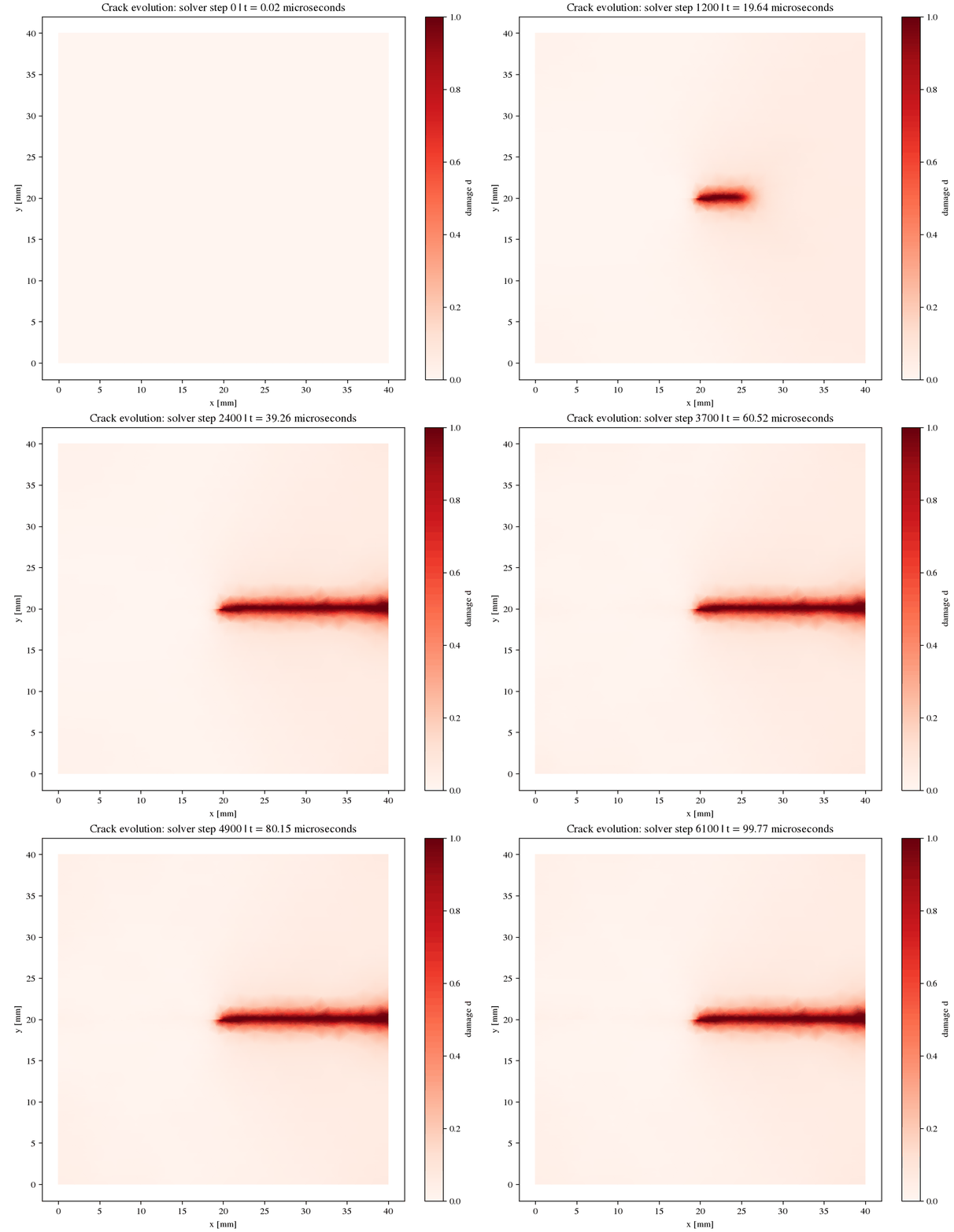
Saved: /home/runner/work/PhAST/PhAST/runs/tutorial_square_plate/crack_evolution.gif
11. Summarize and retain the result
The (x)-extent of nodes with (d\geq0.95) is descriptive. It does not replace a crack-tip algorithm, energy balance, convergence study, or experiment.
high_damage_nodes = coordinates[damage >= 0.95]
if len(high_damage_nodes):
    print(
        "Nodes with d >= 0.95 span "
        f"x = {high_damage_nodes[:, 0].min():.3f} to "
        f"{high_damage_nodes[:, 0].max():.3f} mm."
    )
print("\nTop-level run artifacts:")
for artifact in sorted(RUN_DIR.iterdir()):
    if artifact.name not in {"result.vtkhdf", "training_data.h5"}:
        print(f"  {artifact.name}")
print("  result.vtkhdf     (result file: fields, history, mesh; opens in ParaView)")
print("  training_data.h5  (single-file trajectory store, requested above)")
Nodes with d >= 0.95 span x = 19.644 to 40.000 mm.

Top-level run artifacts:
  config.yaml
  crack_evolution.gif
  damage_final.png
  energy.csv
  final_fields.png
  initial_conditions.png
  mesh.geo
  mesh.msh
  result.vtkhdf.sha256
  run_lockfile.json
  run_metadata.json
  solver_telemetry.csv
  timing_per_step.csv
  result.vtkhdf     (result file: fields, history, mesh; opens in ParaView)
  training_data.h5  (single-file trajectory store, requested above)
Interpretation and limitations
Successful execution demonstrates this workflow for the selected configuration. The cells report which fields were stored, check their finiteness, and print the actual extent of nodes exceeding the stated damage threshold. Cleared notebook outputs make no claim about a previously computed crack path.
Do not infer more than that:
the mesh and time increment have not undergone a convergence study;
the result is not newly compared with the Borden et al. benchmark data;
the compact mesh is instructional, not a publication-quality prediction;
local CPU timing is not a portable performance claim;
changing (G_c), (\ell_0), loading, or mesh defines a new study and requires corresponding resolution and validation checks.
For quasi-static fracture, use
examples/quasistatic/miehe_tension/config.yaml. Do not change only
the solver type here and assume the boundary-value problem remains equivalent.
Suggested student exercise
Predict first, modify one item, and rerun into a new directory:
increase
SNAPSHOT_EVERYto reduce stored trajectory size without changing the solver update cadence; orrefine the mesh and recompute the CFL increment before changing the step count.
If installation, execution, or interpretation remains unclear, open a GitHub issue with the first error, platform, Python version, command, and configuration. Questions, reproducible bug reports, documentation corrections, and student contributions are welcome.